WaterALLOC User Manual

Enrique Triana

Juliana Corrales

Current Version 2.4.1.7

Introduction

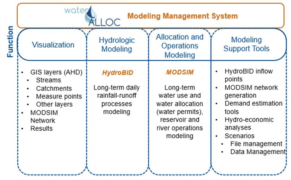
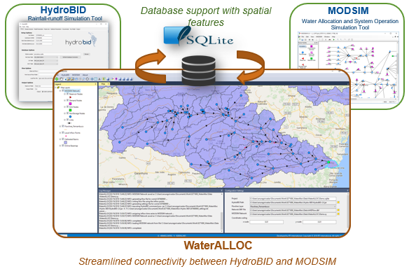
WaterALLOC is a modeling management system that provides a new geographic information system (GIS)-based interface that streamline the data processing between HydroBID and MODSIM models, offering a solution to perform water availability analysis, including river and reservoir operations with simulation of water permits and priorities, using all the river operations tools and customization provided by MODSIM. WaterALLOC was created to enhance the user experience for both, HydroBID and MODSIM users, allowing the HydroBID user to use the GIS interface to run the system and adding easy-to-use input dialogs for agricultural and municipal demands for MODSIM. Additionally, his tool creates the MODSIM simulation network automatically from the Analytical Hydrology Dataset (AHD) network built for HydroBID, using the catchments and streams to define the links and nodes of the MODSIM network.

WaterALLOC links the results of local runoff from HydroBID to the entry nodes of MODSIM to simulate the routing of the flows in the streams of a basin. Georeferenced demand nodes can be created within the WaterALLOC interface to simulate water intake and consumption according to water availability at different points of the basin and in accordance with the permits, priorities, and physical and hydraulic limitations of the system. Also, WaterALLOC allows the creation and simulation of operation of reservoir systems, simulating water supply and power generation operations.

The new robust modeling platform offers a streamlined solution for data management between the models, the ability to perform comprehensive water balance analysis that includes water infrastructure operation rules, water allocation priorities, and administrative and social constraints. Additionally, the platform supports scenario management allowing the simulation and analysis of dynamic changes to land cover, water demands, population, surface and groundwater interactions, and climate.

WaterALLOC Approach

WaterALLOC builds upon two existing modeling tools, HydroBID and MODSIM with the purpose of enhancing the ability and effectiveness in providing streamlined and comprehensive solutions for water resources management around the world. WaterALLOC brings together the hydrologic simulation capabilities from HydroBID and the river basin simulation capabilities from MODSIM to support water resources planning and management.

	HydroBID	MODSIM
Function	Rainfall-runoff processes modeling	River basin operation and planning modeling
Description	Highly scalable rainfall-runoff modeling system model based on the generalized Watershed Loading Factor (GWLF) formulation to estimate the availability of surface water (stream flows) at the regional, basin, and sub-basin scales.	Generic river basin management decision-support system capable of simulating complex, large-scale surface water networks; excels in the area of administering water in systems governed by water rights, administrative constraints, and agreements.
Features	Includes the Analytical Hydrography Dataset for Latin America and the Caribbean (LAC AHD), a digital representation of more than 300,000 catchments with their corresponding topography, river, and stream segments Includes a GIS-based catchments and streams navigation tool Provides a climate data interpolation interface to obtain rainfall and temperature inputs for the area and period of interest Includes a routing scheme for quantifying time of travel and cumulative flow estimates Additional modules: Simulates the effect of climate change Simulate the effect of reservoirs on downstream flows Link with MODFLOW groundwater models to incorporate water exchanges between groundwater and surface water Model sediment loads using Modified Universal Soil Loss Equations	Uses linear-network structure and optimization as an efficient technique to operate the system and allocate water Performs water allocation based on priorities or water rights Includes features for reservoirs operation Allows simulation of stream-aquifer interaction and operations impacts Includes customizable pre-processing, execution, and post processing
Distribution	Publicly available	Publicly available
Developer	RTI International	Colorado State University

WaterALLOC Key Features

• Provides a GIS interface to visualize the catchments, streamlines, MODSIM network and results

• Uses the AHD geo-spatial features to create the MODSIM network

• Allows a full map of the stream network or a simplified network

• Allows launch and run HydroBID and MODSIM from the same interface

• Allows to perform watershed analysis (similar to the AHD Navigation Tool in QGIS)

• Imports the output from HydroBID into the MODSIM network

• Prepares the MODSIM network with HydroBID settings for a ready to run model

• Allows visualizing the HydroBID output spatially in the map

• Allows access to the MODSIM objects, functionalities, and outputs

• Allows creating new features to complete the water allocation analysis (demands and reservoirs)

• Provides statistical metrics and graphs to calibrate the model

• Provides a hydro-economic module to conduct cost-benefit analysis

• Provides a scenario management structure to address “what if” questions and develop and compare scenarios with different assumptions

WaterALLOC Development

Since 2017, RTI has provided primary support for WaterALLOC development through Independent Research and Development (IR&D) Projects. Also, client-driven improvement and software customization has been conducted on project-based cases funded by the Inter-American Development Bank (IDB).

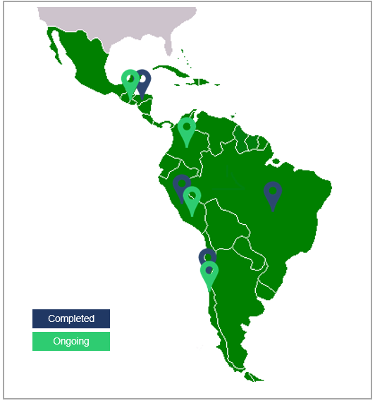
Since its initial development, WaterALLOC has been applied successfully in several countries in the Latin American and Caribbean Region (LAC) to simulate complex hydrological systems, to support long-term planning, and provide a framework for integrated water resources management.

Year	Country	Client	Status	Description
2018	Peru	IDB Invest/ Danper S.A.C.	Completed	Assess water optimization activities for the Peruvian agro-industry company Danper S.A.C. located in Trujillo, Peru. Develop a water balance model to simulate the water supply and demand in the basins where Danper’s agricultural and industrial productions are located. Assess impact on the water balance considering water demand and climate variability to better understand the risk and vulnerability associated with Danper’s operations in the context of climate change. Provide a cost-benefit analysis on alternative technologies that can help mitigate water shortages and optimize the use of water. Identify green infrastructure measures focused on water collection and water storage that could be implemented in areas facing water security issues.
2018	Chile	IDB/Fundación Chile	Completed	Evaluate the impact of climate change on future water balance for the Maule basin.
2019	Brazil	IDB/ ADASA/ANA/ CAESB/SEAGRI	Completed	Support the analysis of water supply planning for the Federal District (FD) by understanding and reducing its vulnerability to severe droughts, and by increasing the efficiency in the allocation of available water resources among different competing users, while providing a decision support tool for water resources management and water allocation. Illustrate the application of hydro-economic tools for determining efficient resource allocation and analyzing tradeoffs among competing water uses in a selected study area.
2020	Honduras	IDB/ UGASAM- SANAA/ENEE	Completed	Analyze the current and future conditions of water availability and scarcity for the city of Tegucigalpa in Honduras in a context of climate change, and to analyze potential water sources and different management strategies to reduce the current water deficit that faces the capital city.
2020	Peru	IDB/SEDAPAL	Ongoing	Support the development of a system for the planning and integrated management of the basins that supply water to the Metropolitan Area of Lima (AML), which will seek to minimize the environmental, economic, and social impacts due to drought events.
2021	Colombia	IDB	Ongoing	Develop technical capacities and apply HydroBID and WaterALLOC management tools to support the formulation of Water Safety Plans for four water utilities under the IDB’s COMPASS program.
2021	Chile	IDB	Ongoing	Support the development of a Drought Management Plan (DMP) for the Maipo basin that will pursue to minimize the environmental, economic, and social impacts of drought episodes.
2021	El Salvador	IDB	Ongoing	Provide capacity building in HydroBID and WaterALLOC modeling tools to assess the current and projected water balance in selected watersheds. Implement a water permit management module in WaterALLOC to assess water availability for existing permits in different sectors, taking into consideration the historical or projected flow regimes in a specific basin.

WaterALLOC Software Installation

WaterALLOC is distributed at no cost to our clients. To install WaterALLOC, copy the installation files into a folder and run the installer by double clicking the setup.exe file and then click on Install in the prompt window.

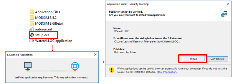
When installation has completed successfully, you can open the program by searching for WaterALLOC in the Start menu of Windows and then clicking on the program icon .

RTI provides a free license to use the software for non-commercial purposes. The license is granted for 30 days and it is automatically renewed with an Internet connection every 30 days.

WaterALLOC runs in Microsoft Windows computers with a minimum of XX RAM capacity and an Internet connection is not required.

Note: Although it is not required to install MODSIM in your computer, several versions of MODSIM are also distributed within the program installation files. Having MODSIM installed can be useful for editing complex networks.

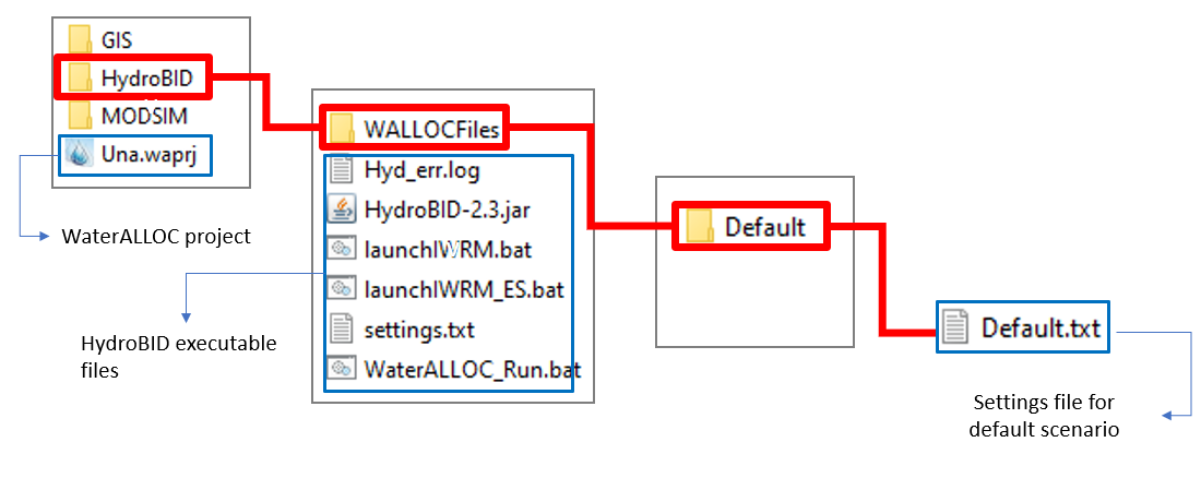
WaterALLOC Workspace

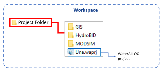
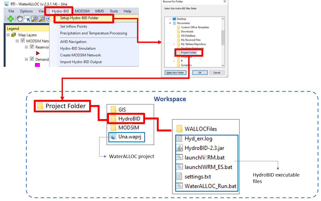
The workspace refers to the location where all inputs files, model executables, databases, and supplemental information related to a WaterALLOC project are saved. In other words, it is the location of the Project Folder. When a new project is created in WaterALLOC, users need to specify the directory of the Project Folder or can make a new folder in a specified location, and the WaterALLOC project file (.waprj) and two subfolders named “HydroBID” and “MODSIM” will be automatically created and saved in the Project Folder. In the HydroBID folder there will be all executable and settings files needed to run the model and a subfolder named “WALLOCFiles” where all HydroBID output files in .csv format will be stored. The HydroBID folder can also be set through the HydroBID main menu in WaterALLOC (see Section 6.2.1). All the MODSIM .xy files used in the WaterALLOC project and the output files (in a sqlite database) will be stored in the MODSIM folder. It is suggested that all the shapefiles that are used in the project are stored in a subfolder within the Project Folder, such as “GIS” to avoid problems with the visibility of the layers uploaded in the map when opening the WaterALLOC project from a different directory or a different computer.

HydroBID and MODSIM Modeling Tools

To get started, we suggest getting familiarized with the following key concepts about HydroBID and MODSIM.

HydroBID Overview

The HydroBID modeling system for quantitative simulation of hydrology and climate change has three primary components: the Analytical Hydrography Dataset (AHD), the database, and the hydrologic model.

AHD

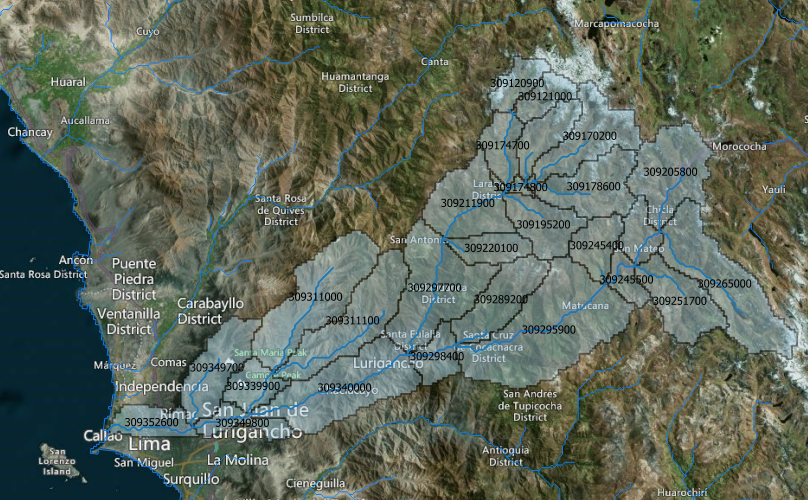
The AHD is a digital representation of catchment boundaries and stream segments for the entire LAC region, containing over 300,000 catchments with an average size of 83 km² for South America and 23 km² for Central America and the Caribbean. The AHD is a regional platform of spatial data used to integrate the disparate data needed to support hydrologic modeling. It provides a framework for consistently parameterizing models, provides the necessary river network connectivity, and stores the data necessary for displaying results in a GIS format (Rineer and Bruhn, 2013).

COMID

Each of the catchments and stream segments delineated in the AHD has a unique identifier number known as COMID, which allows to quickly identify the basins and rivers that drain at a certain point within the extension of the AHD.

AHD Flow Table

HydroBID includes a table containing the upstream/downstream relationship between each stream or each catchment. The table with this information is the AHD flow table (AHDFlow.dbf). This table allows the navigation of the AHD using GIS tools and in the WaterALLOC interface.

Database

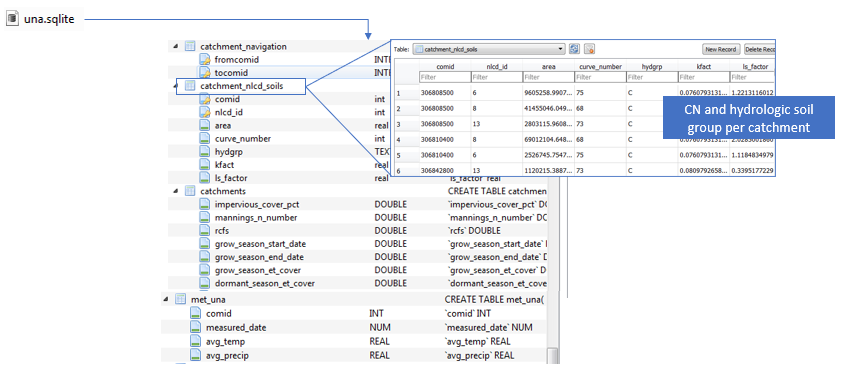
The database contains information associated with each catchment, including drainage area, stream length, slope, land uses, soil types, and climate. Additionally, each catchment in the AHD is parametrized with land use and soil type data from global datasets. The land cover data is based on the U.S. Geological Survey (USGS) Global Land Characterization and the soil type data is based on the Harmonized World Soil Database (HWSD) supported by the International Institute for Applied Systems Analysis (IIASA) and the Food and Agriculture Organization (FAO). The catchment’s soil and land cover conditions determine the Curve Number (CN) and the hydrologic soil group that the model uses to calculate runoff. All the input data for HydroBID, including climate tables, is stored in a single SQLite database.

Hydrologic Model

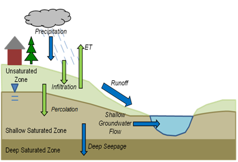
The hydrologic model is an enhanced version of the rainfall-runoff Generalized Watershed Loading Function (GWLF) model (Haith and Shoemaker, 1987), coupled with a novel lag-routing methodology developed by RTI (Moreda et al., 2014). The model computes runoff and baseflow by catchment. The GWLF estimates runoff using the U.S. Soil Conservation Service’s curve number (CN) method. Catchment CNs are stored in the database and are determined by the watershed’s combination of soil and land cover conditions, which are represented as hydrologic soil groups, cover type, treatment, and hydrologic condition. After runoff estimates, excess precipitation infiltrates to the unsaturated layer where it is subject to evaporation. Over time, the infiltrated water percolates from the unsaturated layer downward to replenish the saturated storage. Water within the saturated layer enters the stream channel as baseflow where it combines with runoff from the catchment and any inflows from the upstream catchments to provide the stream flow volume, which is then routed through the stream network defined by the AHD (Add Reference to Technical Note 2).

Climate Data Interpolation Tool

A preprocessor referred to as the Climate Data Interpolation Tool (CDIT), built into the HydroBID modeling system, automates spatial interpolation of daily temperature and precipitation time series between stations. The tool uses the Inverse Distance Weighting (IDW) method to interpolate climate data at the centroid of each catchment.

HydroBID Outputs

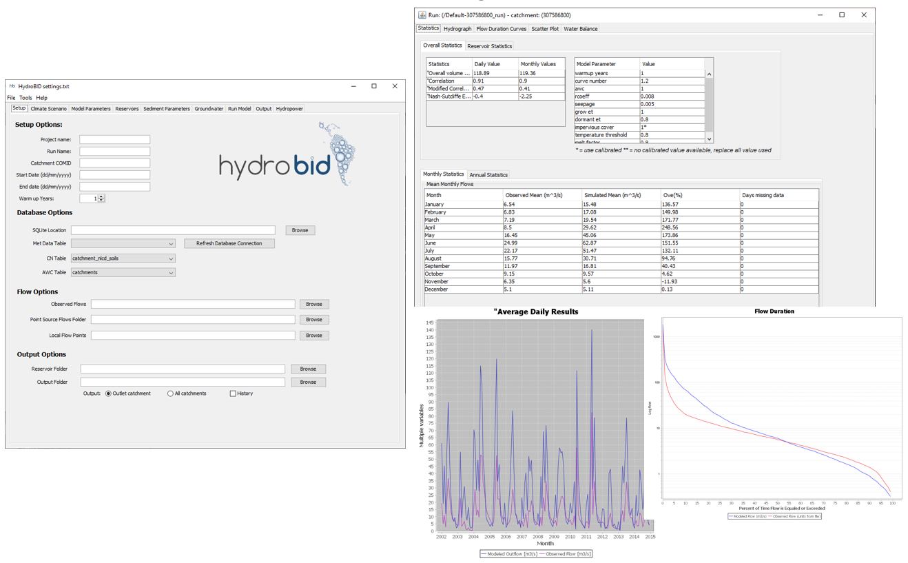
HydroBID can simulate stream flows in unimpaired watersheds for historic, current, and future conditions based on land use, precipitation, and temperature inputs. Model outputs of predicted streamflow are saved in readily usable, comma separated value (.csv) format, at either a daily or monthly time step. The system has a graphical user interface (GUI) to facilitate loading and processing of model input, as well as to display both graphical and tabulated model output.

The hydrologic model utilizes the data structure and the catchment and stream network topologies of the AHD to generate flow estimates at the outlet of any catchment or basin selected by the user. In addition to flow generation, HydroBID includes other modules for 1) reservoir simulation, 2) sediment transport, and 3) surface and groundwater interactions using MODFLOW.

Calibration Parameters

HydroBID contains several calibration parameters that are used to adapt the model and optimize its performance simulating observed streamflows. HydroBID provides default values for some of the hydrologic parameters in the database. For instance, the database contains values for the CN and for AWC in the vadose zone. However, these parameters need to be calibrated to historical streamflow measurements by modifying a factor that multiplies the values already contained in the database. For other parameters, such as the recession (r) and seepage (s) coefficients, the user needs to enter the initial values that will be applied uniformly to all catchments within the simulated area.

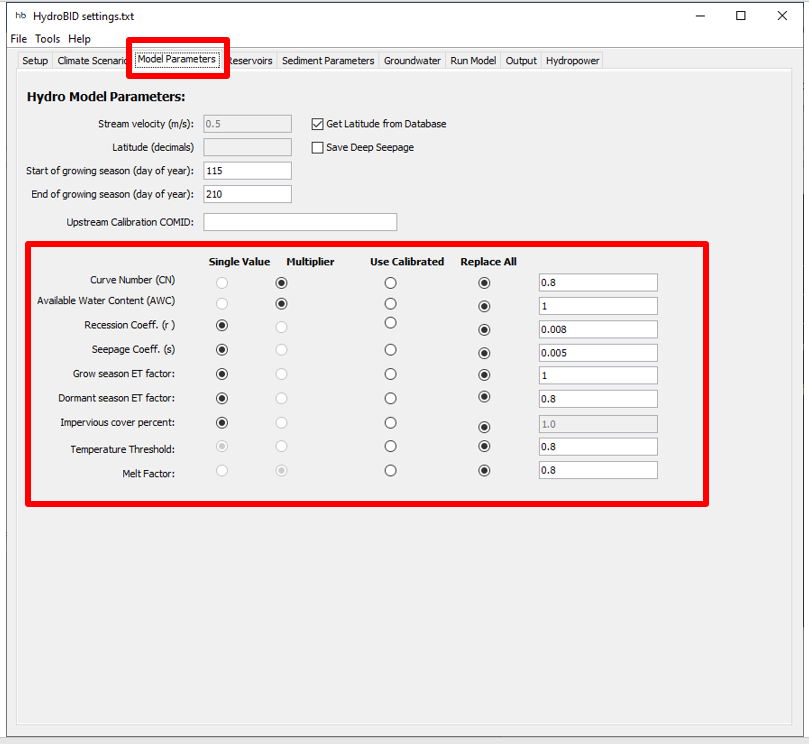
The table below provides a list of the calibration parameters and the suggested value range.

Parameter	Description	Suggested Value Range
Curve Number (CN)	Controls the initial amount of abstraction used to calculate runoff. Default values are available in the database.	0.8–1.2 (multiplier)
Available Water Capacity (AWC)	Enables the start of percolation from the unsaturated layer to the saturated layer. Default values are available in the database.	0.2–1.2 (multiplier)
Recession Coefficient (r)	Control base flow rate.	0.001–0.75 (day-1)
Seepage Coefficient (s)	Controls the rate of percolation to the deep saturated zone.	0.005–0.1 (day-1)
Evapotranspiration Factor (ET) in the Growing Season	Evapotranspiration factor during the growing season.	0.5–1.5
Evapotranspiration Factor (ET) in the Latent Season	Evapotranspiration factor during the dormant season.	0.5–1.5
Temperature Threshold	Temperature below which precipitation is assumed to be snow and above which accumulated snow will melt.	-1–4 (°C)
Melting Factor	Factor controlling the rate at which snow melts.	0.3–0.6 (mm day-1 °C-1)

Settings File

HydroBID saves all the setting parameters provided in the GUI into a text file (.txt). This setting file allows an identical re-run of the model at any time in the future. When open HydroBID, the GUI will be automatically populated with the values in the setting file, and all required data for a model run will be obtained from the current folder.

MODSIM Overview

MODSIM, developed by the Colorado State University, is a decision-making support system that uses optimization in a stream network to help watershed managers with the analysis of water supply in the face of hydrological uncertainty and demand growth (http://modsim.engr.colostate.edu/). As a decision support system, MODSIM is designed for developing improved strategies for short-term water management, long-term operational planning, drought contingency planning, water rights analysis and water allocation between urban, agricultural, and environmental sectors (Labadie, 2012). The model uses the concept of flow networks to efficiently simulate complex water systems at river basin scale.

One of the advantages of MODSIM is that it can be customized for any unique basin management conditions, specialized operating rules, input data, output reports, and access to external models running concurrently with MODSIM, all without having to modify the original MODSIM source code. In addition, RTI holds a collaboration agreement to support the maintenance and development of MODSIM and provide our clients with enhanced and long-term support.

Below are some of the key MODSIM capabilities. Labadie, 2012 has a complete list of the software capabilities.

Network Flow Optimization

The basic solver in MODSIM is a state-of-the-art network flow optimization algorithm that is more than an order of magnitude faster than solvers currently in use in other river basin modeling packages and capable of modeling extremely large-scale networks. The optimization of stream network provides an efficient way assuring allocation of flow in accordance with specified rights and priorities.

Data-driven Model

MODSIM maintains complete reliance on user input data and specifications for describing system features, operational requirements, and priorities, which are separated from the network modeling algorithmic structure. No a priori defined operating policies or priorities hardwired into MODSIM.

Long-term Planning to Real-time Operations

MODSIM is applicable to long term planning (monthly), medium term management (weekly), and short-term operations (daily) in river systems.

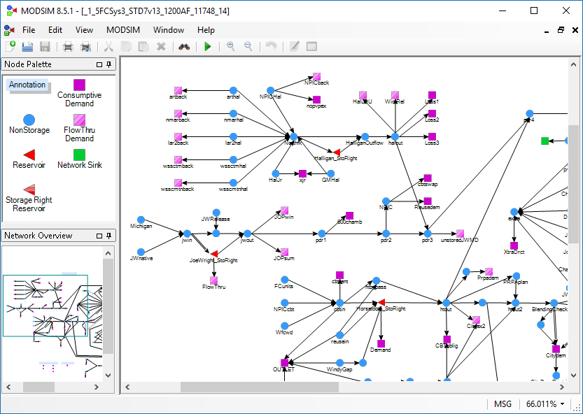
Complex River Basin Configurations

Complex network topologies can be constructed, including looped and bifurcating flow paths. Network topology is graphically created by simple point and click actions on the GUI palette. In addition, georeferenced network topologies can be loaded into MODSIM from a geographic information system (GIS).

Reservoir Operations and Hydropower Generation

Reservoir balancing routines are included, allowing division of reservoir storage into several operational zones for controlling the spatial distribution of available storage in a river basin. Hydropower generation capacity and energy production is based on power plant efficiencies varying with discharge and head. Energy production calculations are performed, with consideration of tailwater effects and head-dependent hydraulic capacity restrictions on reservoir discharge.

Conjunctive Use

MODSIM includes modeling capabilities for conjunctive use of surface water and groundwater and simulation of stream-aquifer interactions. A stream aquifer model based on the USGS sdf approach is included, as well possible linkage with external groundwater models.

Water Rights and Storage Contracts

MODSIM is capable of directly incorporating institutional structures governing water allocation under direct flow or natural streamflow rights and seasonal storage rights and contracts, including provisions for allocating water according to specified priorities based on current river basin conditions.

Customized MODSIM

Users are provided access to all key variables and object classes in MODSIM, thereby allowing customization for any complex river basin operational and modeling constructs without the need for reprogramming and recompiling the MODSIM source code. Custom code can be developed for defining complex operating rules and policies, executing external modules such as water quality models, input of specialized data sets for particular applications, preparing customized model output and reports, and linking MODSIM with database management systems to provide access to timely data and forecast information for real-time river basin management.

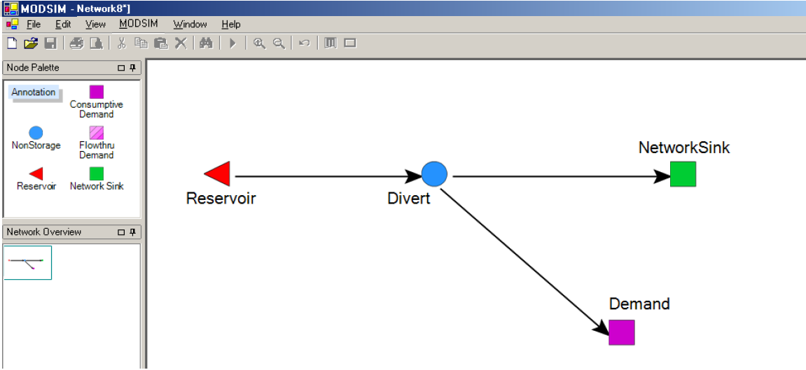
The physical water resource systems are represented as a network of nodes, both storage (i.e., reservoirs) and non-storage (i.e., stream confluences, diversion points, and demand locations), and links (i.e., canals, natural river reaches).

Some of the key characteristics and example applications of MODSIM are:

Features

Selected Application Examples

Uses linear-network structure and optimization as an efficient technique to operate the system and allocate water Performs water allocation based on priorities or water rights Includes features for reservoirs operation Allows simulation of stream-aquifer interaction and operations impacts Includes customizable pre-processing, execution, and post processing

Long-term water supply planning: “Planning under deep uncertainty” Evaluation of salinity recovery strategies Analysis of alternative infrastructure option for water supply Water rights yield and third-party effects Investigation of impacts of ecological flows enforcement Optimization of reservoir operations, including hydropower Water availability studies for operation expansion or sustainability

WaterALLOC Features and Functionalities

WaterALLOC GUI

The WaterALLOC interface consist of a map window to visualize the physical features of the study area and the MODSIM network elements; a main menu at the top, providing access to HydroBID and MODSIM functionalities; a toolbar menu that provides one-click access to various GIS and other program functions; a log messages window that records all the actions performed by the user and also shows error messages; a project settings window that is used to set the configurations of a WaterALLOC project and allows access to scenario management and view; and a layer explorer panel shown in the left side of the interface that allows to hide/show all layers available and to customize their properties.

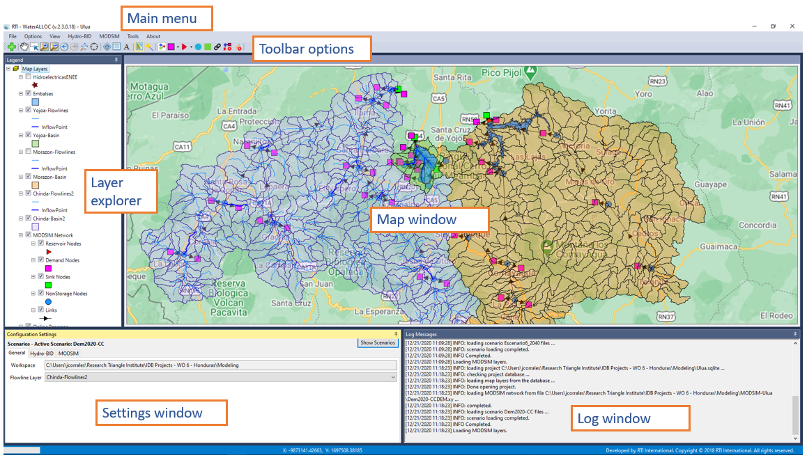
Main Menu

The main menu provides access to the most important functions of WaterALLOC.

• File: Allows to create a new WaterALLOC project, open an existing project, and save changes made to a project.

• Options: Allows to switch between English and Spanish languages and to activate WaterALLOC modules, such as the hydro-economic module.

• View: Allows to activate the different windows of the WaterALLOC interface.

• HydroBID: Allows access to the AHD Navigation tool, which allows to navigate downstream/upstream the catchments and river segments and perform a watershed analysis, to the HydroBID simulation to set the configurations of the model run (i.e., sqlite, climate data, observed streamflow files, calibration parameters, etc.) and view the results. Also, allows access to the create MODSIM network and import HydroBID output windows.

• MODSIM: Allows access to MODSIM network settings and to run the model.

• MMS: Allows access to the optimization module.

• Tools: Allows to import a layer from a comma separated value (.csv) file.

• Help: Includes the license agreement and the WaterALLOC version, and allows access to the user manual.

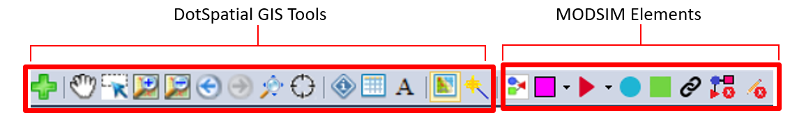
Toolbar Menu

The toolbar menu provides access to some GIS functions and MODSIM available elements.

This Icon	Is Used to:
	Add layers to the map
	Move the map to progressively display adjacent areas
	Select objects displayed in the map window. To select an object, make sure to select the layer in the Layer Explorer Panel on the left.
	Zoom in the map
	Zoom out the map
	Zoom to the previous extent
	Zoom to the next extent
	Zoom to maximum extent
	Zoom to coordinates
	Identifies features of the selected object in the map
	Show the attribute table of selected layer. Also allows to query the selection of features
	Select label
	Enable/disable basemap
	Select local inflows
	Enable/disable MODSIM layers
	Demand Node. Add consumptive demands (i.e., agricultural, domestic, groundwater pumping). Demand nodes can also be added by importing a shapefile or a .csv file
	Reservoir Node. Add reservoirs for modeling reservoir storage operations and hydropower generation
	Nonstorage Node. Simulate catchment runoff, which are imported from the outputs of HydroBID. Add tributary inflows, water transfers, groundwater return flows
	Sink Node. Basin outlet
	Link. Add maximum and minimum flow, stream channel losses
	Remove MODSIM nodes and links
	Stop editing mode

Project Settings Window

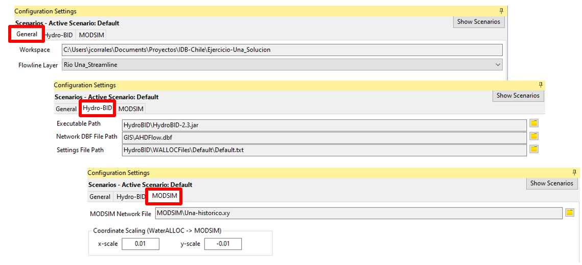
The settings or project preference window shows the active scenario in the WaterALLOC interface and provides the absolute or relative paths to the configuration files of a WaterALLOC project and scenarios. It is divided in three main tabs:

• General tab shows the absolute path to the workspace and allows to select the flowline layer.

• Hydro-BID tab shows the relative paths to the HydroBID .jar (executable) file, the AHD Flow table, and to the HydroBID settings file.

Note: When creating a WaterALLOC project (.waprj), a HydroBID folder is automatically created in the same workspace, which includes HydroBID executables and a WALLOCFiles subfolder that organizes outputs files of HydroBID runs for different scenarios. Also, a folder for the Default scenario and its respective settings file is automatically created.

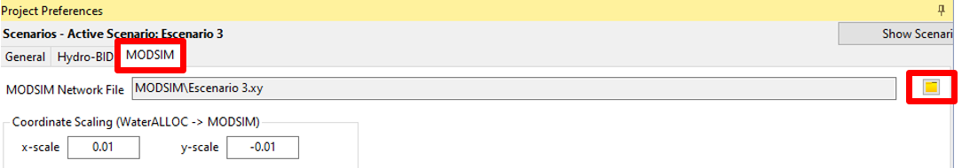
• MODSIM tab allows access to an existing MODSIM network file or allows to create a new .xy file. It also allows to modify the coordinate scaling factors, which are used to convert the GIS coordinates to the MODSIM interface canvas.  Depending on the GIS projection used, the user might have to experiment with the convenient set of values to comfortably display the network in MODSIM.

The project settings window also allows to hide/show the scenarios management panel. See Section 6 for more information about the scenario management.

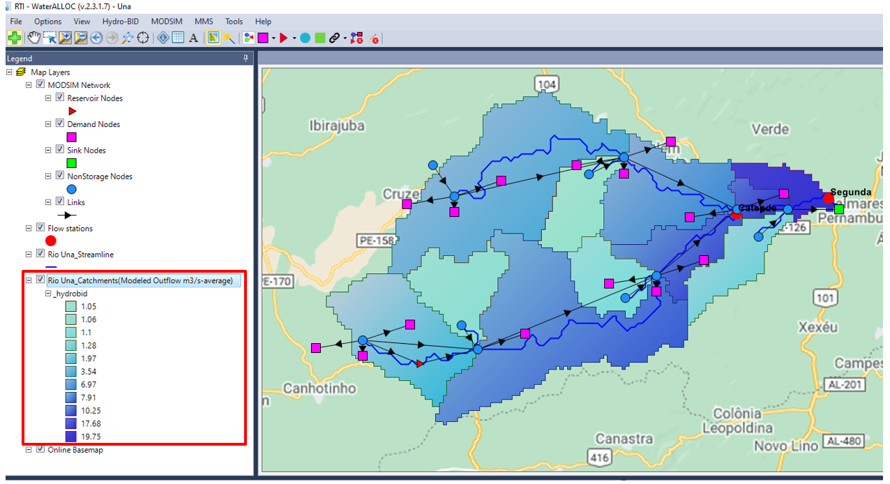
Layer Explorer Panel

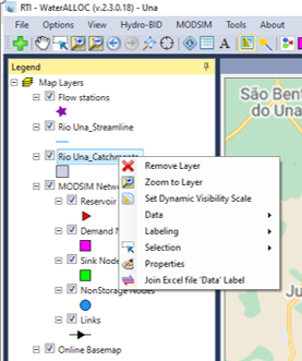
All layers added to a WaterALLOC project will be displayed in the layer panel on the left. The panel helps manage the display order of map layers and their symbology and set other properties of each map layer. Layers listed at the top are displayed first, followed by the layers below them. A layer’s attribute information can be accessed by clicking the attribute table icon ( ) or the Identifier icon () in the toolbar menu. When creating a WaterALLOc project, the MODSIM Network layers and the Online Basemap are automatically loaded to the panel. These layers should not be removed. Use the check box to the left of each layer to turn it on or off. Right-click on the layer to zoom to layer, export all or selected features, set labels, and access the Properties dialog window to change the symbology.

HydroBID Tools

WaterALLOC offers different HydroBID tools that can be accessed through the HydroBID main menu. Below, there is a description of the functionalities of each of the HydroBID tools.

Set up HydroBID Folder

This option will prompt a window where the user can navigate to the workspace or project directory and set a HydroBID folder. A folder named “HydroBID” will be created, and the model executables files together with a WALLOCFiles subfolder will be automatically saved within this folder.

Set Inflow Points

The Set Inflow Points tool allows flagging inflow points in the flowline layer. It creates a field named IsFlowPnt in the attribute table of the flowline layer shapefile.  The tool needs a field COMID to identify the objects to flag. The field IsFLowPnt is created the first time that the tool is used, if it does not exist. The tool stacks the map selected features in the "Selected COMIDs" list and provides the buttons to add and remove the listed features from the list of inflow points. The “Label” is automatically filled in, adding the sufix “_Inf” to the COMID. The label can be edited by the user. The Label is used to name the MODSIM non-storage node representing the inflow point.

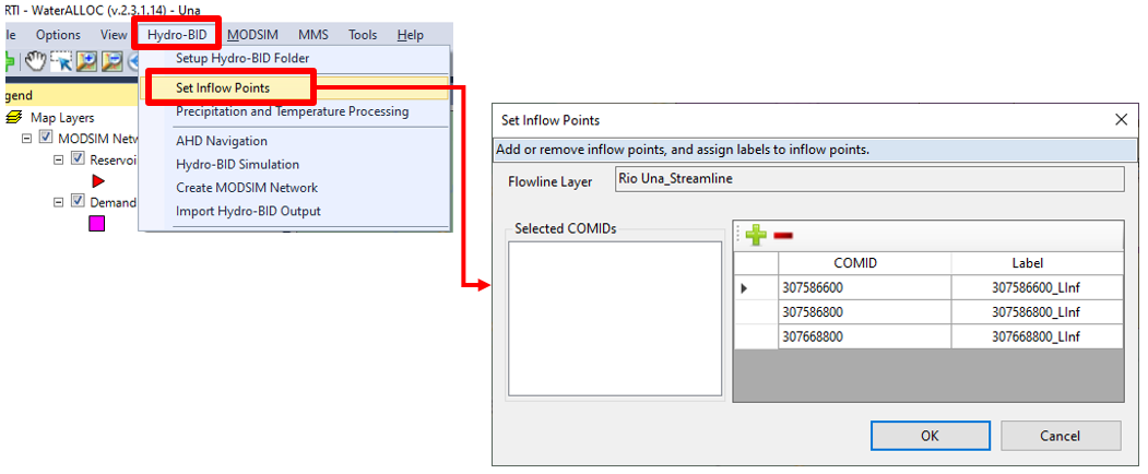
Once inflow points are set, the properties of the streamline shapefile can be changed to display Inflow Points in different color and width using the Highlight Inflow Points icon ().

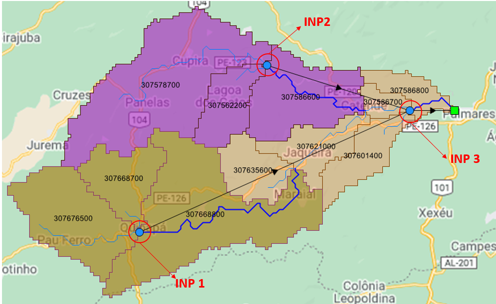
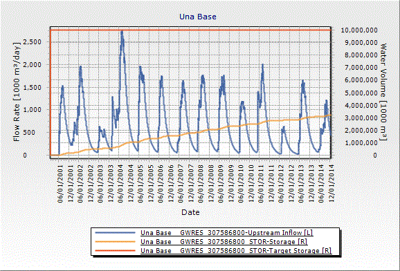
The flow simulated at the Inflow Points is the aggregate flow of all upstream catchments (COMIDs) plus the flow of the catchment where the inflow point is selected. For instance, from the figure below the flow at each of the three Inflow Points (INP) is mathematically represented as follows. Note that the colors of the catchments represent the area that contributes to a specific INP.

Flow at INP 1 = Flow_307676500 + Flow_307668700 + Flow_307668800

Flow at INP 2 = Flow_307578700 + Flow_307562200 + Flow_307586600

Flow at INP 3 = Flow_307635600 + Flow_307621100 + Flow_307601400 + Flow_307586700 + Flow_307668800

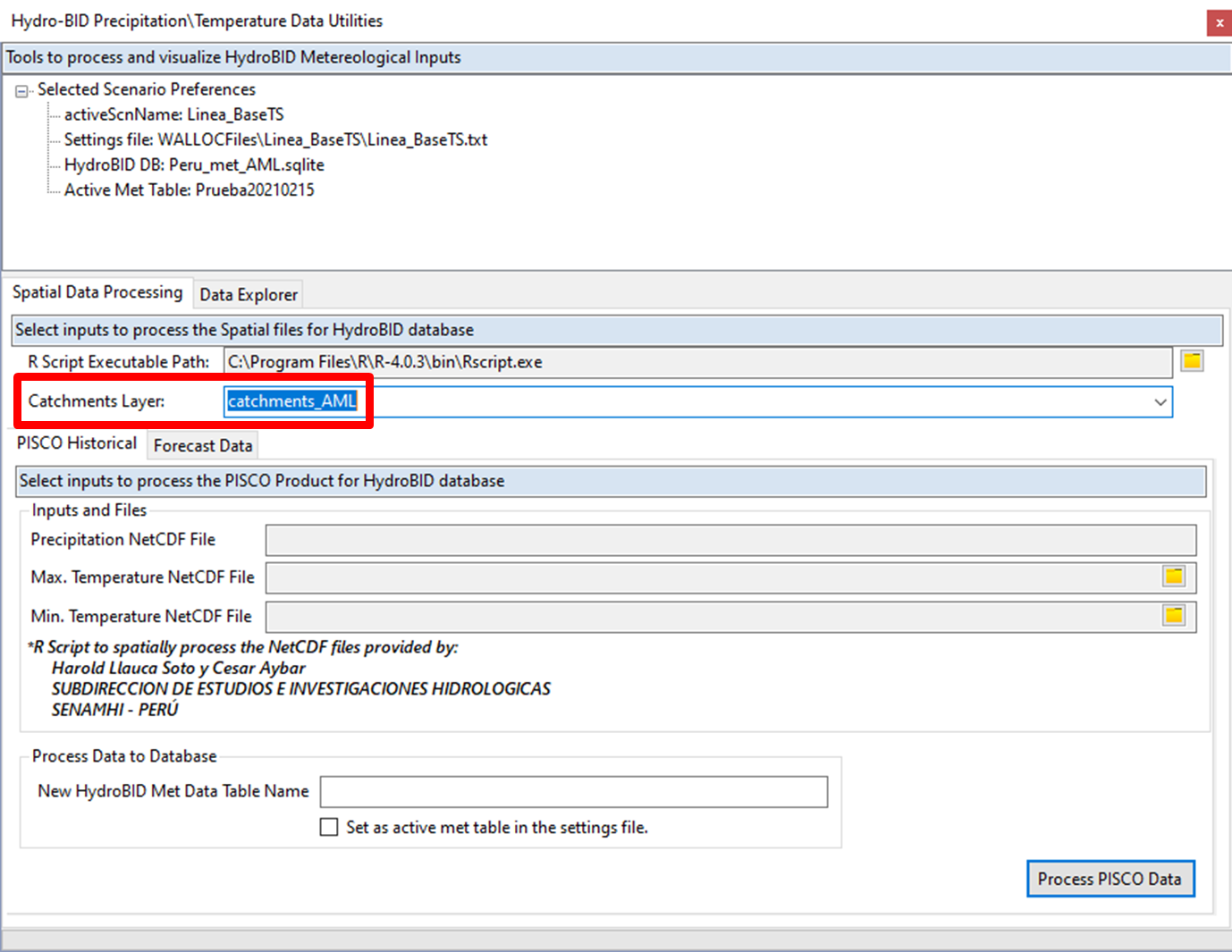
Precipitation and Temperature Processing

These set of tools allow processing and visualizing the HydroBID meteorology data in the HydroBID database. The spatial processing tools allows calculating mean aerial estimates of precipitation and temperature for each catchment in the study area and summarize the results into the HydroBID database. The spatial data processing tool includes a historical data processing mode and a forecast data processing mode. The visualization tool displays the available datasets in the database and allows generating plots and tables of the precipitation and temperature time series for each of the catchments, identified by the COMID. User interface uses the current scenario HydroBID settings file to load the data available in the referenced database.

Spatial Processing of Historical Data

The spatial processing is performed using an R script that performs the areal operation. R needs to be installed and operational in the computer to perform these tasks in WaterALLOC. The path of the R executable is preset in WaterALLOC to the default location, however, if R is installed in a different location, it can be selected using the browse button. The spatial data processing is performed for the selected Catchments Layer domain. The data in the NetCDF rasters should cover the Catchments Layer extends.

Spatial Processing of Forecast Data

Data Visualization

[Work in progress - ET]

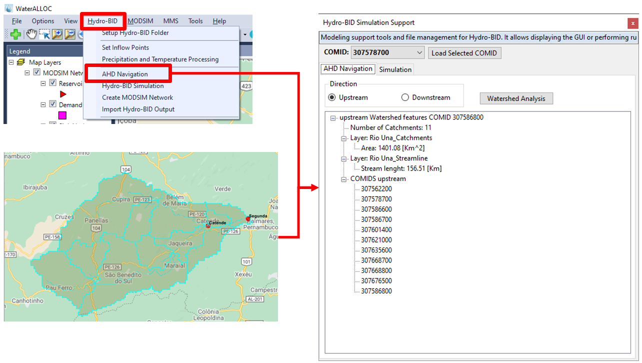
AHD Navigation

WaterALLOC includes a tool that allows to browse AHD catchments and streams with the capability of navigating upstream and downstream and selects a set of catchments that belong to a given watershed. This AHD Navigation Tool is useful to identify the drainage area of a basin for simulation, for which the tool requires the identification of the most downstream AHD catchment. Once the downstream catchment is provided, the system navigates the database (AHDFlow.dbf) and collects all the catchments within the basin. The tool is run through the “Watershed Analysis” button and yields information about the count of catchments navigated, total area in square kilometers, the length of all flowlines in kilometers, and provides a list of the COMIDs of all catchments selected.

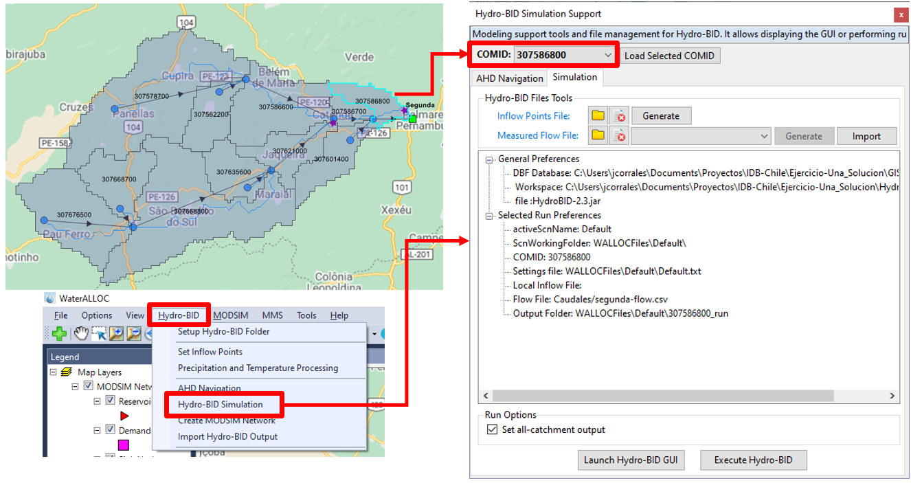
HydroBID Simulation

HydroBID is a standalone program written in Java but can be launched and run through the WaterALLOC GUI using the HydroBID Simulation tool. The user needs to identify the most downstream catchment (COMID) of the basin that will be simulated in HydroBID. Additionally, observed flow time series can be imported to an existing link in the MODSIM network to facilitate comparison with the simulated flows. The inflow point files can also be search for or generated.

Once the COMID has been selected or loaded, the HydroBID Simulation window shows general preferences, such as the location of the AHD flow database and the workspace, and preferences for the selected scenario, including the settings file, flow file, and output folder. Users have two options to run HydroBID. The first option is by launching the HydroBID GUI using the button “Launch Hydro-BID GUI” and the second option is by executing the model in a batch mode with the “Execute Hydro-BID” button. The first option enables to make changes to the configurations (e.g., changing calibration parameter values) before running the model, whereas the second option runs the model with the configurations in the settings file. The option “Set all- catchments output” might be selected to obtain outputs for each of the catchments within the simulated basin.

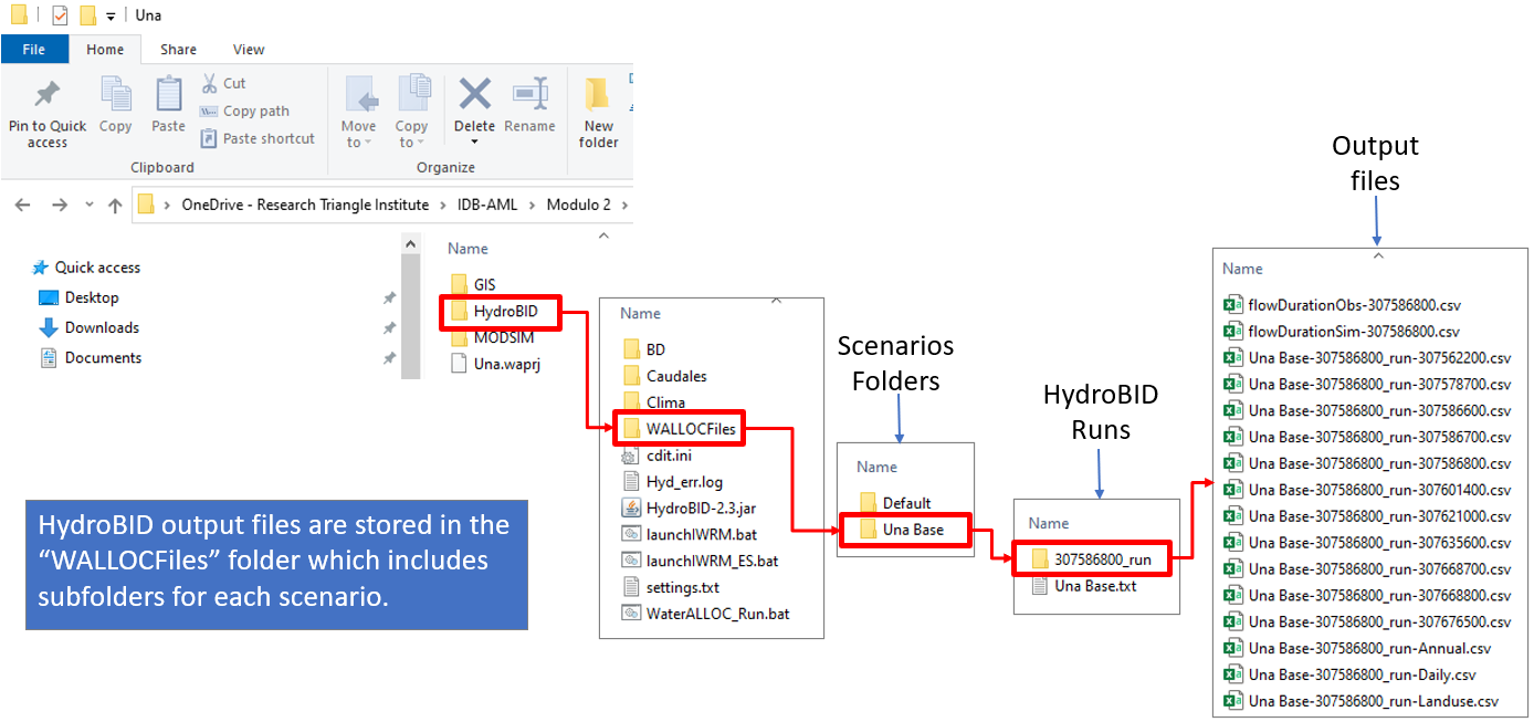
Once HydroBID is run successfully, the output files are stored in the WALLOCFiles folder and in the folder for the active scenario. WaterALLOC populates the output file names for the HydroBID runs using the scenario name and the COMID.

Create MODSIM Network

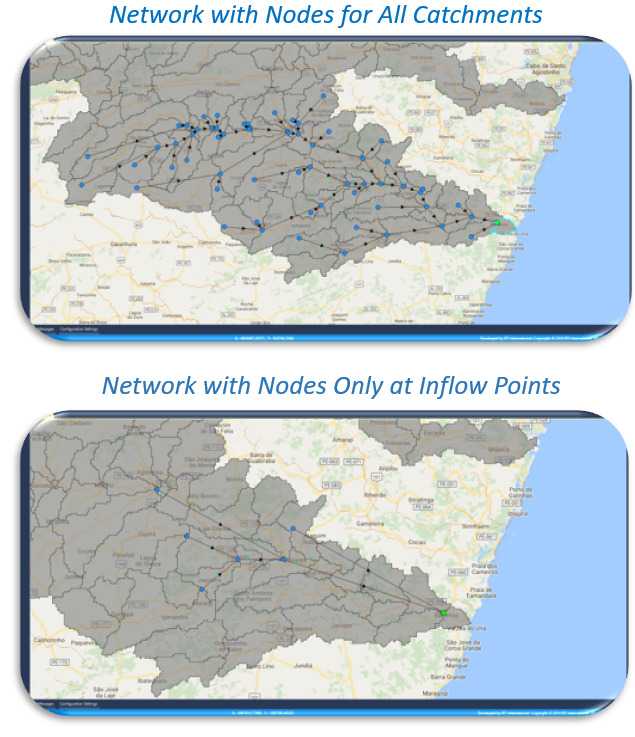
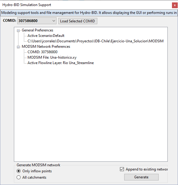
The Create MODSIM Network tool offers two options to automatically create a MODSIM network that represents the simulated basin. The “All catchments” option creates a network with inflow points (Nonstorage MODSIM nodes) for all the catchments within the study area. This option allows to create a network that matches the AHD stream network. On the other side, the “Only inflow points” option allows creating a simplified MODSIM network with only the local inflow locations (previously identified with the Set Inflow Points option) representing the hydrologic inflows (NonStorage nodes). The latter option is useful when simulating big watersheds where there is no need to have a detailed network and inflows can be aggregated at key locations.

To create a MODSIM network, the most downstream catchment needs to be selected. In the dialog window, the COMID of the catchment is visible, and general and MODSIM network preferences are shown, such as the active scenario, path of the workspace, name of the MODSIM file, and the streamline layer. Additionally, the window includes the option to append a network to an existing MDSIM network. If the “Append to existing network” is uncheck, WaterALLOC will replace any current network with the newly created.

Import HydroBID Output

One of the main functionalities of WaterALLOC is streamline the connection between HydroBID outputs and MODSIM inputs to provide efficiency in the use of the combined features of both models. Through the Import HydroBID Output tool, users can import outputs from HydroBID into the MODSIM network. The available output to be imported will be shown in the window, which is tied to the active scenario in the WaterALLOC GUI. Available outputs appear in different rows and can be identified by the RunName.

There are several output variables than can be imported. In the To MODSIM tab, the tool will import the “Generated Flow m3/day”, which refers to the simulated flow generated at each catchment, to the MODSIM network. When MODSIM is executed, flows will be then routed through the hydrologic network until reaching the Sink node. When importing outputs for “All catchments”, HydroBID had to be run for all catchments, so each of the catchments has its respective output file. If the “Overwrite MODSIM Settings” option is selected, the MODSIM Network Settings (e.g., time step and simulation period) are replaced with the configuration in the HydroBID setting file. Note that once simulated flows are imported, units are adjusted to the MODSIM default units (1000 m³/day).

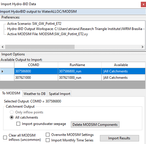
In addition to importing the Generated Flow simulated in each catchment, this tool allows to import groundwater seepage simulated also with HydroBID, which can be used to approximate the underneath aquifer recharge. When the option “Import groundwater seepage” is selected, WaterALLOC processes the HydroBID seepage into the MODSIM network. The first time this option is used in the network, it creates a MODSIM reservoir at the catchment selected to be imported to simulate the aquifer water balance and connects each catchment upstream with the reservoir to simulate the groundwater seepage (i.e., deep percolation) as a daily volume of water, multiplying the seepage depth by the area of the catchment, which is taken from the Catchment Shapefile and the Area Column field specified by the user. The processing of seepage creates a set of inflow nodes to capture the percolation and convey it to the reservoir node that simulates the groundwater storage. These inflow nodes and the reservoirs are connected with links in a separate MODSIM layer called “WAlloc_GWSeepage”, that can be turned on/off in the “Visible MODSIM Layers” check list.

Once the network includes the seepage network construct nodes and links, the HydroBID import tool can import the surface water runoff only or both the surface runoff and the seepage to the MODSIM inflow nodes. In the case the seepage links exist and the use elects to not include the seepage, these links will be closed during the import operation and only surface water runoff will be processed to the non-storage inflow nodes.

Overwrite MODSIM Settings: When activated will use the simulation preferences defined in HydroBID to set the MODSIM simulation period and daily time step. It will also assign an accuracy of two decimal digits by default.

Import Monthly Time Series: When activated it will process the daily HydroBID results into a monthly time series with average flows (m3/day) for the entire month. This option should only be used if the MODSIM simulation is intended to be in a monthly time step.

Clear all MODSIM inflows: This option will clear all the non-storage nodes inflow time series in the entire network (not only the basin to be proceeded) before processing and importing the HydroBID time series. Caution should be used in multi-basin MODSIM networks to avoid losing other flows imported into the network.

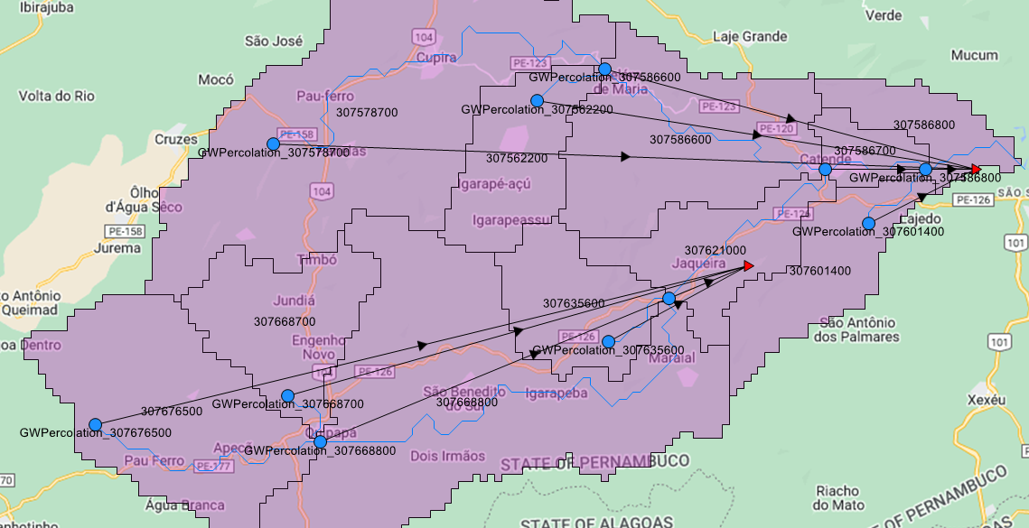
Results simulate natural recharge to the aquifer (represented with the reservoir node) from natural processes. The Upstream Inflows to the reservoir collect the total natural aquifer recharge simulated by HydroBID. The non-storage nodes created in this operation for each sub-watershed are independent of the surface water inflow nodes with the prefix “GWPercolation_” and the corresponding COMID.

Note multiple aquifers can be created in the study area. They should be created from upstream to downstream. The downstream groundwater reservoir only connect to sub-catchments that are not already connected to an aquifer reservoir.

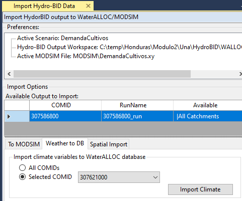
In addition to import outputs to MODSIM, the Weather to DB tab allows to import weather data from the HydroBID database to the WaterALLOC database for all catchments (all COMIDs) or for a selected COMID. This is useful when estimating net water demand for irrigation, so agricultural demand considers the precipitation data used in HydroBID to estimate the irrigation requirements. The precipitation imported will be provided as options in the agricultural demand nodes regardless of the spatial location.

Furthermore, the Spatial Import tab allows to import any HydroBID output variable to be visualized in the map window of the WaterALLOC GUI. This feature enables to visualize the spatial distribution of modeled flows and other output variables within the basin.

MODSIM Tools

Creating MODSIM Networks

There are different ways to create MODSIM networks to work with WaterALLOC: 1) using the HydroBID AHD, 2) using a shapefile with unique identifiers, and 3) loading a previously created MODSIM network. The first option is described in Section 6.2.6. The second option can be accessed through the MODSIM main menu and then selecting Network Utilities. This option needs a shapefile with a unique field (e.g., COMID) and a filed with the drainage area. These two fields need to be selected in the Create Network tab. The drainage area information is stored in the project database (.waprj) in a table called “wateralloc_runoffSupp”. This table is associated with each scenario and contains the MODSIM GUID associated with the element originally created and the associated drainage area. When user click on the “Create Network” button, the tools will create a non-storage node for each unique feature in the shapefile.

A simplified network can also be created in the Topology Tools tab, using inflow points previously set with the Set Inflow Points tool.

Explain about Network Adjustments tab….

The third option to create a MODSIM network in waterALLOC is loading a previously created network. In the tab MODSIM in the Project Preference window, users can navigate to a specific MODSIM file (.xy) by clicking in the yellow folder icon.

Setting MODSIM Elements

Once a MODSIM network is created in WaterALLOC representing the natural hydrologic dynamic of the basin, the network can be complemented with other MODSIM elements, such as demands and reservoirs, to characterize different interventions, developments, and operations occurring within the basin.

The WaterALLOC GUI provides spatially referenced capabilities that allow to add and link basin network elements on the display, and then populate data for that element by right-clicking to open the dialog window form associated with that element. The Toolbar Menu at the top of the GUI contains several MODSIM elements icons, such as demands, reservoirs, non-storage, and sink nodes for adding them in the network by clicking on the icon and then clicking on the desired location in the Map Window.

Demands

There are three options to parametrize water demands ( ) in WaterALLOC:

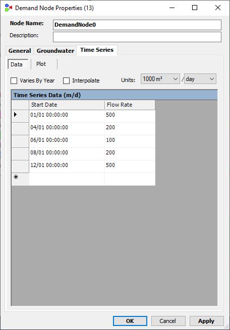
• Option 1: Manually through the demand node properties dialog

Right clicking on a demand node and selecting “MODSIM” opens a dialog window of the node properties. In the "Time Series" tab, the volume of water used can be added, which can be defined as historical diversions, water concessions, agricultural, municipal and industrial demands based on consumptive use calculations carried out outside of MODSIM.

The demanded water volume can be entered manually or by copying and pasting the time series. Selecting “Varies By Year” allows to enter time series for different years; not selecting it allows demand patterns to repeat annually. There are other complex operations, such as groundwater pumping, infiltration, and return locations that can be set through the node properties window as well.

• Option 2: Manually through the WaterALLOC data entry dialogs

  • Add mathematical equations to calculate demands using data input through WaterALLOC dialogs

WaterALLOC displays data entry dialogs that allow to parametrize agricultural and municipal water demands by clicking in the “Agriculture” or “Domestic” options at the node. Data entered in the dialog windows is used to calculate the volume of water demanded for MODSIM runs.

• Agriculture Demands can be defined by “User Defined” crop parameters or by “Crop-based” default parameters stored in the WaterALLOC database (.waprj).

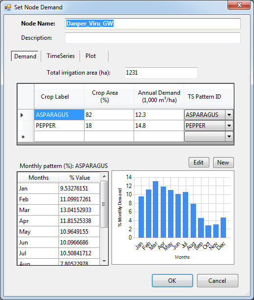
The “User Define” option allows to estimate agriculture demand using the following parameters, per crop (one node can be composed by a single or multiple crops).

• Total Irrigated area (ha)

• Crop label

• Percent of crop irrigated area (%)

• Total annual demand (in thousand cubic meters per hectare - 1000 m³/ha)

• Monthly distribution of annual demand (%/month). There are two default monthly patterns for corn and wheat crops, which can be edited or used to create new ones.

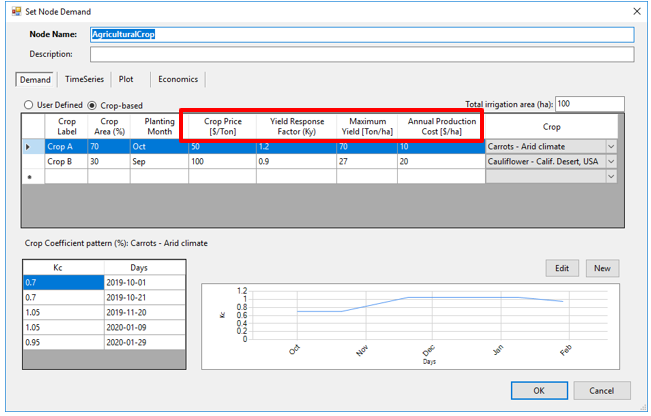
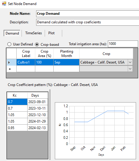
The “Crop-based” option allows to estimate agriculture demand based on preset crop water requirements for different growth stages, which are stored in the WaterALLOC database (.waprj). Users can select a crop from the dropdown menu list and the crop coefficient (Kc) values and planting month will be automatically loaded in the dialog window. The list of crops, their respective Kc values, and development stages were obtained from Allen et al. (1998) and are stored in the WaterALLOC database in the “wateralloc_croptype”, “wateralloc_cropcoeffic”, “wateralloc_cropdevelopmentstage” tables, respectively.

The user-input required data are:

• Total irrigated area (ha)

• Crop label

• Percent of crop irrigated area (%)

This option also allows to input parameters used in the Hydro-economics Tools, such as crop price, yield response factor, maximum yield, and annual production costs.

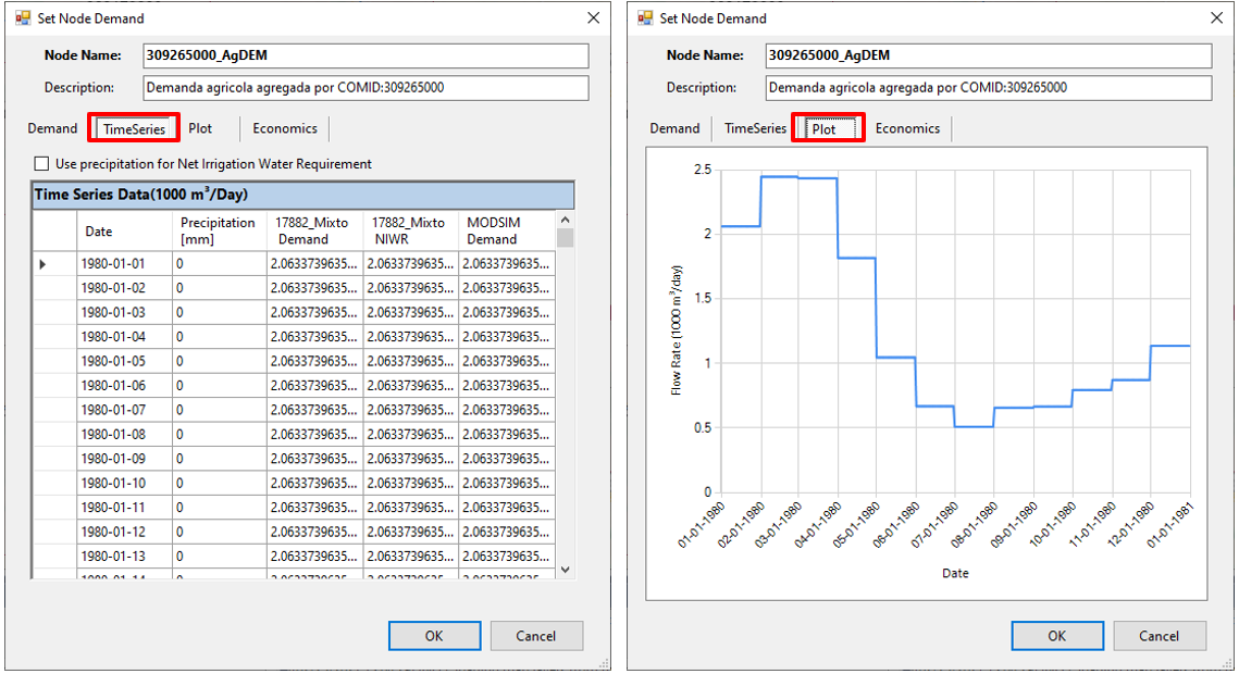
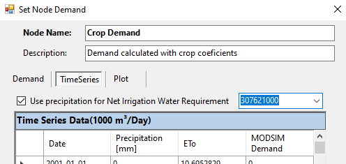
The net irrigation water requirement (NIWR) for the node is computed using the input parameters, and is shown in table and graphical formats, under the “Timeseries” and “Plot” tabs, respectively. When the “User Defined” option is selected, precipitation data from HydroBID are made available to compute the portion of the water requirement supplied by rain; the remaining water required is the NIWR for the node. Precipitation time series are imported when HydroBID is executed and stored in the WaterALLOC database to be available to the demand nodes. The combined NIWR for all the crops in a demand node becomes the MODSIM demand, that is, water that is requested from the stream network and allocated by MODSIM based on priorities and simulation of operations.

• Municipal Demands can be defined by four user-input parameters. Each raw in the dialog window can represent a municipality, city, town, district, or zone (i.e., urban, suburban, rural).

  • Total population

  • Area label

  • Percent of population area (%)

  • Total annual demand (gallon per capita per day - gpcd)

  • Monthly distribution of annual demand (%/month). There is a default monthly pattern for household, which can be edited or used to create new ones.

The WaterALLOC Agriculture and Municipal dialog windows also show the total water demand for the node calculated using the input parameters, in table and graphical formats, under the “Timeseries” and “Plot” tabs, respectively.

For Agricultural demands, WaterALLOC offers the option to

Weather variables from Hydro-BID are made available to compute the net irrigation water requirement (NIWR).  These variables are imported when Hydro-BID is executed and stored in the WaterALLOC database to be available to the demand nodes.  The weather is selected in the demand nodes in the 'Time Series' tab, along with the option to enable NIWR calculations

• Option 3: Automatically through the WaterALLOC Demands Import tool

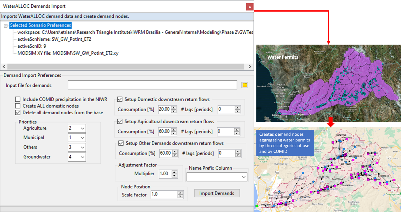
This option is useful for large networks with numerous demands (e.g., water permits). Instead of adding and parametrizing each demand node individually, clicking on the black arrow next to the demand icon in the Toolbar Menu and then on “Import with WaterALLOC Demands Data…” displays the Demands Import Tool dialog window that automatically creates and imports demand data into a MODSIM network to be visualized in the Map Window of WaterALLOC. The tool processes individual water rights by COMID, importing each water right to the agricultural and domestic WaterALLOC demands. Each water rights is imported as an element of the demand and results in a single MODSIM node for each water use type, i.e., agricultural, domestic and other. This tools also allows importing groundwater water rights if the aquifer reservoirs are used in the MODSIM network (See Import groundwater seepage in the Importing HydroBID results section). These groundwater water rights are identified specifying an aquifer as the source and are also added the WaterALLOC demands and combined with the surface water rights. Groundwater water rights can be specified a pumping capacity, which is aggregated per aquifer source for each COMID, and a seasonal capacity as annual pumping limit. The tool preserves existing elements of the network and creates demand nodes by three types of uses (agricultural, municipal, or others) and by COMID. The preferences of the active scenario are shown in the tool, including the MODSIM .xy file.

Demand data needs to be prepared and organized in a comma separated value (.csv) file, which requires the following parameters.

Note: Column labels in the file need to be exactly as appears in the table. The file may contain additional information, but it requires data for the 10 required input parameters.

Parameter	Column Label in the .csv File	Column setting in .csv file
Unique identification number for each water permit	OBJECTID	Required
COMID where the water permit is diverted from (can be obtained with GIS spatial analysis tools, and can include any non-storage node name)	COMID	Required
Type of use (Agricultural “Agrario”, municipal “Poblacional”, and others)	Uso	Required
Integer number from 1 to 4, where 1 is assigned to the water use type with the highest allocation priority and 4 to the lowest.	Prioridad	Conditional
This field includes the maximum flow that can be diverted for each row (or water right) in liters per day. The sum of these values for each demand node is set as the capacity of the link that diverts water from the surface system. The sum is calculated only for demands that do not have specified the “Acuifero”,i.e., surface water source.	Caudal Concesionado (lpd)	Conditional
This is a text field that contains the name of the aquifer that the demand takes water from, and flags demands with groundwater source. The demand is processed with the demands of the COMID non-storage node. When blank or empty, it is assumed that the demand is from the surface.	Acuifero	Conditional
Specifies the pumping capacity for groundwater demands, in liters per day. This value is used to set the flow rate capacity of the link. If multiple groundwater demand are specified for the same COMID, the pumping capacity is aggregated per aquifer (source).	Capacidad Bombeo (lpd)	Conditional
Annual demand (m3)	Demanda Anual (m3)	Required
Type of crop	Cultivo	Required
Irrigated area (ha)	Area irrigada (ha)	Required
Population	Poblacion	Required
Agricultural demand per hectare (1000 m3/ha)	Demanda Anual Ag (1000 m3/ha)	Required
Percent of the annual water use per month (%). These values are used to calculate the water su patterns for the crop and population demands.	%Volumen_1, %Volumen_2, %Volumen_3,… …%Volumen_12	Required
Volume of water used per month (m3/month). These values are used in groundwater demands to set the annual pumping limit (Seasonal Capacity). Seasonal capacity import assumes that the MODSIM is in metric units since the imported values is in 1000 of m3.	Volumen_1, Volumen_2, Volumen_3,… …Volumen_12	Required
Name prefix can be specified in a user defined column. This prefix is added to the name of the demand nodes imported into the model.	[User Defined heading]	Conditional

The import to the WaterALLOC database is only carried out if types of use “Agrario” and “Poblacional” are specified in the csv file under the column “Uso”. These types of use import crop and population data to calculated water demands. For all other uses the specified monthly time series are directly imported to a separate MODSIM node.

The created demand nodes are labeled using the “Uso” column in the csv file and are proportionally distributed around the Non-Storage node from which they take water. The column “Prioridad” is used to assign the cost among the water permits. For those water permits that have a priority assigned in the csv file, the value in the column overwrites the selected values in the Demands Import Tool interface. If the water permit has not a value assigned in the “Prioridad” column, then the values selected in the Demands Import Tool interface will prevail.

Below is an example of a water permits data organized with the required headings.

The Demands Import Tool dialog window also allows to set the priorities for the type of nodes. A value of one (1) means the highest allocation priority and a value of three (3) the lowest. The link cost is calculated using the link number, which is unique, and an equation (Equation 1) that creates 3000 range of cost for each water use type. times the priority number specified by the user in the import tool. This results in unique costs in the ranges of 3000 for each water use type. Note that ground water sources are also included in the cost assignment allowing setting groundwater pumping priority against surface water.

Link Cost = -((5 – UserPriority * 3000) – LinkNumber) Equation 1

Furthermore, the tool provides options to configure return flows, which is useful for modeling efficiency in irrigation and municipal water distribution systems. For instance, a 60% consumption with a lag time of seven (7) days for agricultural demands, means that 40% of the allocated water is returned to the network within the next following seven days.

The tool allows applying a factor to the demand imported to simulate demand sensitivity analyses. A prefix can be specified by the user in a column in the csv file. This text will be appended at the beginning of the standard name of the demand nodes imported.

The node position factor is used to control the distance around the surface diversion node where the demand nodes are created. The smaller the factor, the closest to the diversion point the demand nodes will be created.

[Explain all the features included in “Set Demands” option under the MODSIM main menu.]

Reservoirs

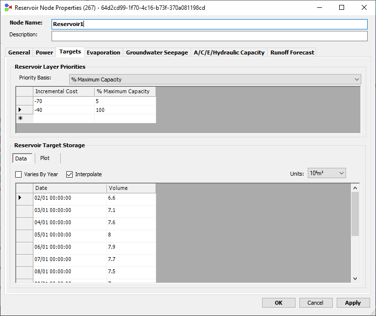
The red triangle node ( ) is used to represent reservoirs in a MODSIM network. The reservoirs can be parametrized with the following key characteristics.

Required	Optional
Maximum and minimum volume Initial volume Reservoir target storage	Evaporation rate Groundwater seepage rate Area/Capacity-Elevation curve Hydropower characteristics

The of Reservoir Target Storage represent the top of the active or conservation storage pool of the reservoir. MODSIM allows the conservation pool to be divided into several operational zones which serve to improve regulation of storage levels in multi-reservoir systems. In addition, the Reservoir Target Storage is used for calibrating MODSIM by specifying target storge levels as measured historical data and then adjusting different model parameters to match observed streamflow records. To achieve relatively balanced storage among several reservoirs in a basin, each reservoir should have the same priority (set in the General tab) and similar incremental costs (se in the Targets tab under Reservoir Layer Priorities).

Users have the option to enter net evaporation rates in the Reservoir Node Properties window, which are defined as evaporation rates minus rainfall rates. Negative entries signify that rainfall rates exceed evaporation rates for that time period. MODSIM accepts a variable number of elevation-area-storage-hydraulic outlet capacity data points for any reservoir, which are interpolated to calculate reservoir surface area corresponding to any current volume in the reservoir. Evaporation loss is calculated in MODSIM as a function of average surface area in a reservoir over the current period (refer to MODSIM user manual for more details).

Seepage is assumed to be a function of average volume in the reservoir over the current period and the seepage loss rate is assumed to be constant. In contrast with evaporation losses, a portion of reservoir seepage may be contributed to downstream return flows. The seepage loss fraction is entered in the Groundwater Seepage tab. Entry of aquifer parameters or return flow lag coefficients allows calculation of downstream return flows from reservoir seepage.

Delete MODSIM Elements

Any MODSIM element can be deleted with the () button. To delete an element, make sure to select the layer of the element that needs to be deleted in the Layer Explorer Panel in WaterALLOC to avoid simultaneously deleting multiple elements. When unwanted elements have been removed, make sure to click the () button to stop the editing mode on WaterALLOC.

MODSIM Network Settings

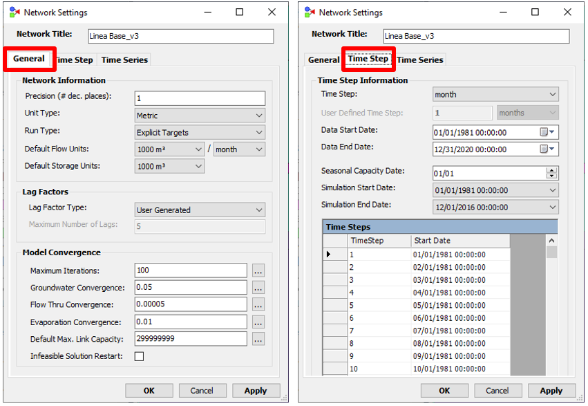
MODSIM network settings can be accessed through the MODSIM Main Menu. In the General tab, users can specify a number of options. For instance, they can select the desired accuracy for data input and flow results can be either integer accuracy or 2-place decimal accuracy. Users can select either English or metric units, with the default units used for storage, flow, head, net evaporation rates and hydropower specified. However, users may input data in any desired units in the node and link properties windows, and MODSIM will automatically convert the data to the default units.

The Time Step tab allows to specify either monthly, weekly, or daily simulation

time steps. Start Date and End Date for time series data entered into MODSIM must

be the same for all data including inflows, demands, reservoir storage targets, etc.

However, a MODSIM simulation run can start and end at any intermediate dates, as

specified in the Simulation Start Date and Simulation End Date. This is useful, for example, when calibrating the model using a subset of the historical data set.

Cost Analysis

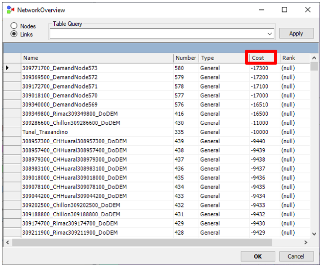
The Cost Analysis option under the MODSIM Main Menu displays the Network Overview form providing a tabular listing of all nodes and links in the network. Clicking the radio button next to Links lists all links and gives information on the link Type and Cost and clicking the radio button next to Nodes lists all demand and reservoir nodes and gives information on the node Type and Priority. The form provides a convenient way, particularly for large networks with numerous demand and reservoir nodes, to edit Node Priorities or Link Costs without having to select the node object in the WaterALLOC Map Window and display its properties form. In addition, a number of Table Queries are available for displaying only those nodes that satisfy particular criteria for evaluation.

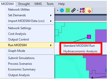
Run MODSIM

Once the system network has been created and the database populated, MODSIM can be executed from the WaterALLOC interface under MODSIM > Run MODSIM. The “standard MODSIM Run” is the default MODSIM run and should be used when there are not extensions selected. The “Hydroeconomic Analysis” run is only displayed when selecting the “Hydro-Economics” extension under the Main Menu Option > Extensions. The later option should be used only when applying the Hydro-economic Tools.

MODSIM Priorities to Allocate Water

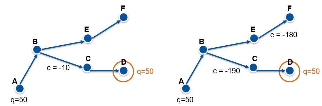
In MODSIM, optimization is primarily conducted as a means of accurately simulating the allocation of water resources in accordance with operational priorities based on system objectives, operational experience, water rights, and other ranking mechanisms, including economic factors. The objective function in MODSIM is set to minimize the product between the flow rate (q) and cost (c) (weighting factors, or water right priorities per unit flow rate) in all links. The Cost defines the preference or priorities for moving water. Rather than their absolute values, it is the relative order or ranking of the negative costs that determines how MODSIM allocates network flows. It is important to note that the solution accumulates costs in the network for flow paths. For example, in the two networks below, the amount of water (q=50) available at the non-storage node A will primary flow the path towards node D because the cumulative cost of the links between nodes A and D is higher than the cumulative cost of the links between A and F.

Hydro-economics Tools

To support hydro-economic analysis, RTI developed a module that leverages the WaterALLOC user environment and database to organize and store the economic data. It uses the MODSIM customization features to perform economic benefit calculations based on the MODSIM water allocation simulation, and it leverages the MODSIM output system to store the results of the economic analysis for each time step. The result is a module that integrates inputs, output, and scenario management through the WaterALLOC interface.

The hydro-economic methods implemented in WaterALLOC considers three main water use sectors: agriculture, municipal supply, and hydropower. For each type of water use, the model estimates, in monetary terms, the benefits of water use. More precisely, it estimates the net benefits associated with the amount of water supplied to each water user to fulfill the sector’s purpose, because it also allows the user to account for and deduct the costs associated with each water use activity.

Sector	Net Benefit
Agriculture	Revenue from crops produced with irrigation, net of production costs
Municipal Supply	Value of water supply to domestic users, net of delivery costs
Hydropower	Revenue from electricity generation, net of operation costs

Given these sector-specific benefits, the model then estimates the aggregate (i.e., combined) benefits of any user-specified water allocation scenario, by summing net benefits across the different water uses and nodes within the system. These aggregate benefits can be estimated for each period specified in the model and can be further aggregated across periods and expressed as a present value.

Therefore, the model provides results that allow the user to directly compare the aggregate benefits of different water allocation scenarios. In other words, the user can see how aggregate benefits increase or decrease from one allocation scenario to another.

In addition, this module allows users to assess the cost–benefit implications of specific projects that permit different water allocations within the system. For example, it can be used to assess infrastructure projects that expand irrigated area or improve irrigation efficiency. For these types of applications, the user specifies the main cost components for the project (e.g., capital, operation and maintenance [O&M]) and the corresponding water allocation, and the model generates results comparing the present value of project costs with the present value of changes in aggregate water use benefits.

Agricultural Sector

For the agricultural sector, WaterALLOC allows defining the water needs as a function of one or multiple crops in a water demand node, using two options: 1) the user can specify the annual crop water requirement and a monthly pattern for each crop, or 2) specify the crops with their associated irrigated area to estimate the crop water requirement based on the crop growth stages and characteristics.

Crop Water Requirement

WaterALLOC assumes that the crop water requirement (ETc) can be supplied by rainfall, irrigation, or a combination of the two. The calculation uses daily rainfall from a user-specified precipitation time series to estimate the portion of the water requirement supplied by rain, while the remaining water required is the net irrigation water requirement (NIWR) for each crop. The combined NIWR for all the crops in a demand node becomes the MODSIM demand, that is, water that is requested from the stream network and allocated by MODSIM based on priorities and simulation of operations.

While in option 2, ET_c is provided by the user, under option 1, ET_c is calculated using the following equation:

ETc = KcET0	Eq. 1

Where:

K_c is the crop coefficient (unitless), which varies by crop type, climate, soil evaporation, and crop growth stages. Use and typical values of this coefficient can be found in Allen et al. (1998).

ET_o is estimated crop reference evapotranspiration and is estimated using the Blaney–Criddle equation, which is a function of the temperature and daytime hours (Allen and Pruitt, 1986):

ETo = p(0.457Tmean + 8.128)	Eq. 2

T_mean,\ is the mean daily temperature (°C) as the average of the maximum and minimum temperatures.

p is the mean daily percentage of annual daytime hours.

This option requires the user to import weather variables (i.e., temperature, precipitation, and daylight hours) from HydroBID into the WaterALLOC project (database) and the selection of a precipitation time series, which are imported associated with a HydroBID COMID.

The weather variables are imported to the WaterALLOC database using the HydroBID Import Data feature, selecting either all COMIDs or a selected COMID. [1]

Once the weather variables are imported, they become available in the WaterALLOC demand estimation tool and can be used to calculate the demand based on the user-defined crop and irrigated area. To estimate the demand, in the WaterALLOC Agricultural demand user dialog select the cultivated crops and corresponding areas.

Then, in the TimeSeries tab, select the COMID with the weather variables to be used for the calculation.

Crop Annual Yield Function

Y_x\ is the (maximum) annual crop yield (in ton/ha/year), when the crop water requirement is fully met over the growing season. This maximum yield is considered a local factor because it depends of multiple factors, including soils, practices, climate, and others, and it is usually obtained from historical production records. Y_a is the actual annual crop yield (in ton/ha/year), depending on the actual water applied and effective rainfall. Vaux and Pruitt (1983) define the relationship between the maximum yield and the actual yield as:

(1 − Y_a/Yx) = K_y(1 − ET_a/ETx) Eq. 3

Where:

K_y is the crop yield response factor (unitless), representing the effect of a reduction in evapotranspiration on yield losses. The K_y concept and application guide can be found in Steduto et al. (2012)

ET_a is the actual annual evapotranspiration (in meters) and is represented by the water received by the crop from both rainfall and irrigation.

ET_x is the annual crop water requirement that yields Y_x (in meters). This value is assumed to be equal to ET_c when no water constraints exist.

For each crop, for the irrigated area in the demand node, the yield function as a function of the volume of water required and supplied in a year can be written as:

	Eq. 4

Where:

A is the irrigated area for this crop (in hectares).

S_i is the supply from surface irrigation simulated in MODSIM for this crop for day i in .cubic meters Note there could be multiple crops in the same demand node, so the total supply to the demand node is distributed proportional to the irrigated land included in the node.

Pp_i is the precipitation for day i (in cubic meters per hectare).

D is the number of days in the year.

Economic Benefit

With the annual production Y_a (tons/ha/year) for each crop, the economic benefit (net benefit in monetary units) is calculated using the market crop price, the production costs, and the area irrigated for each crop.

NetBenefit = (Y_a(P) − (C_p))A Eq. 5

Where:

P is the crop market price (in monetary units per ton).

C_P is the cost per hectare per year to produce the crop, including O&M and irrigation costs.

User Inputs in WaterALLOC

The user input to evaluate net benefits include, for each crop:

• Crop price ($/ton)

• Yield response factor (Ky)

• Maximum yield (tons/ha/year)

• Annual crop production cost ($/ha/year)

These inputs are provided by demand nodes that represent a single or a collection of agricultural water demands.

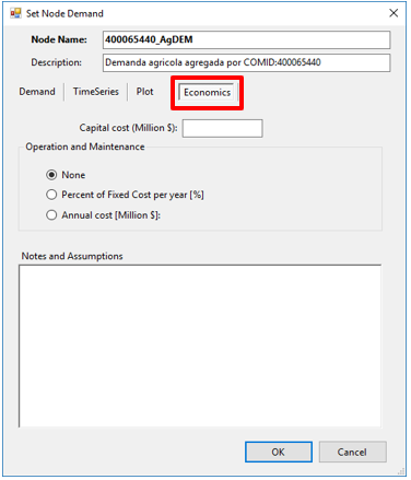
In addition, for each node, the user can include cost components for water projects that will affect the supply or demand for water in the agricultural sector. In particular, the user can specify: 1) the “capital cost,” representing the one-time costs incurred in the initial stage of a project and 2) O&M costs representing the ongoing costs incurred annually for the life of the project. O&M costs can be defined either as fixed annual monetary value or as a percentage of the capital costs.

Municipal Sector

For public water supplies, the benefit from providing potable water to residences is represented using estimated economic demand curves for water, combined with cost estimates for alternative sources of water.

Unlike the water “demand” terms previously used in this report to describe a fixed amount of water required by a user group, the economic demand curve for water is a functional relationship (D) representing the amount of water that a household k would be willing and able to purchase during a time period t (w_kt), depending on the unit price, P_t (e.g., $/m³), as follows:

wkt = D(Pt, xtk)	Eq. 6

Where:

x_tk is the vector of household characteristics affecting water demand and willingness to pay (WTP) (e.g., income, household size, the existence of a connection to a sewer network)

Rather than a fixed amount, the quantity demanded from an economic perspective varies with respect to price (i.e., higher price entails lower quantity demanded).

In addition to representing the quantity demanded at each price, the demand curve also defines the economic benefits of water received at the point of use. In particular, it represents the maximum amount that households are willing and able to pay for each incremental unit of water. This “marginal” WTP typically decreases with each incremental unit.

Therefore, for individual households, the benefit of water is calculated as the integral under their economic demand curves for water, which can be calculated by:

bwtk(wkt) = ∫〖Pt(wtk,〗xtk)dwtk	Eq. 7

Where:

b_wtk are the benefits (in monetary terms) to household k in period t for a change in water consumption (w_kt).

P_t (w,x) is the function representing the household’s maximum marginal WTP for water (inverse of the water demand curve)

To specifically estimate the benefits of publicly supplied water to households, it is also important to consider the costs to households from receiving water from other sources. Eq. 6 and Eq. 7 represent households’ water demand and benefits from all available sources. In effect, the cost of water from other sources acts as an upper bound on households’ WTP (economic benefit) for publicly supplied water.

Linear Water Demand Curve

In a simple case with linear demand, the household demand and corresponding WTP function (dropping the k subscript for simplicity) would be:

wt = a + bPt + cxt Pt = (wt − (a + cxt))/b	Eq. 8 Eq. 9

where a, b, and c are preference parameters that could, for example, be estimated using regression analysis. In this linear case, the benefits to a household of gaining access to the public water supply system are represented in figure below:

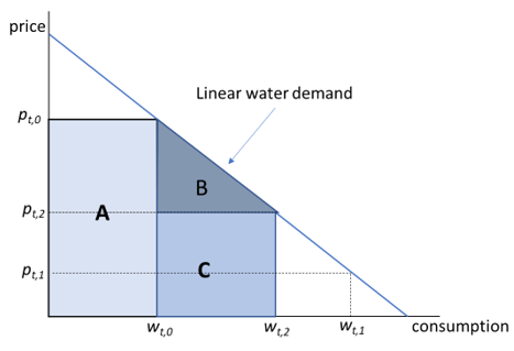
In situations where households lack or have insufficient access to a public water distribution system, it is assumed that the household can pay a price of p_t,0 for water from alternative sources, such as private vendors (including the economic cost for fetching/buying/storing water). If water is only available at this price, then the demand curve implies that a household would consume w_t,0 per period t.

With access to the public water distribution system, if the price per unit of water through the public system is P_t,1, then the household’s water demand during period t would be w_t,1. The amount of water available to the household from the public system (w_t,2) could be less, equal, or greater than w_t,1, and the benefits will be calculated as a function of the water available as follows:

• If w_t,2 ≤ w_t,0, then the household’s benefit is the avoided expenditure on water from the other source.

bt = w(t, 2) * P(t, 0)	Eq. 10

• If w_t,1 > w_t,2> w_t,0, then the household’s benefit is the sum of areas A, B, and C shown in the figure above, where A is the avoided expenditure on water from the other source and B+C is the gross benefit of the difference between w_t,2 and w_t,0.

bt = (w(t, 0) * P(t, 0)) + [(P(t, 0) − ((w(t, 2) − (a + cxt))/b)) * ((w(t, 2) − w(t, 0))/2)] + [(w(t, 2) − w(t, 0)) * ((w(t, 2) − (a + cxt))/b)]	Eq. 11

• If w_t,2> *w_t,1, then the household will consume w_t,1 (the amount demanded at P_t,1*) and the benefit can be expressed as:

bt = (w(t, 0) * P(t, 0)) + [(P(t, 0) − P(t, 1)) * ((w(t, 1) − w(t, 0))/2)] + [(w(t, 1) − w(t, 0)) * (P(t, 1))]	Eq. 12

In each case, the net benefit of public water supply to the household, nb_t, can then be calculated by deducting the variable delivery costs of supplying water to the household. Variable costs refer to those costs, such as pumping costs, that depend directly on the quantity of water supplied.

nb_t = b_t − (c * w_t)

where c is the average per-unit water delivery cost ($/m³).

The aggregate net benefit of water supplies can therefore be estimated by summing household-level net benefits across all affected households. It can be represented as:

	Eq. 13

Where:

K is the total of households

Hyperbolic Water Demand Curve

An alternative simple form for the demand curve, which is implemented in the WaterALLOC economic module, is a hyperbolic demand equation. In the same way as described above, the benefits can be calculated as the area (integral) under the demand curve for water. In a case with hyperbolic demand, the aggregate water demand and corresponding marginal benefit are:

Demand Curve: Inverse Demand (marginal benefit) curve:	Eq. 14 Eq. 15

Where:

W_t is the quantity of water demanded/consumed by all households in period t.

P_t is the price per unit (m³) of water in period t.

α and β are coefficients of the aggregate demand function, and β represents the price elasticity of water demand.[2]

The figure below shows the hyperbolic demand curve with the areas to calculate the benefits for the different supply scenarios (above).

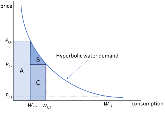
In this case, if, for example, the amount of public water available to households is increased from W_t,0 toW_t,2, the aggregate benefit, B_t,\ is calculated as the integral of the demand curve (i.e., Area B + Area C).[3]

	Eq. 16

To estimate the aggregate net benefit of the change in public water supply, the costs of the additional water supplied must be deducted. This can be done using the average per-unit cost as follows:

NBt = Bt − (c * 〖[W〗t2 − Wt0])	Eq. 17

User Inputs in WaterALLOC

The user inputs to evaluate aggregate benefits of public water supply include:

• Demand curve parameters (β and α or P_t,1)

• Alternative supply price (P_t,0).

• Estimating net benefits requires an estimate of the average per-unit cost c.

In addition, for each node, the user can include cost components for water projects that will affect the supply or demand for water in the municipal sector. As with agricultural projects, the user can specify 1) the “capital cost,” representing the one-time costs incurred in the initial stage of a project, and 2) O&M costs representing the ongoing costs incurred annually for the life of the project. O&M costs can be defined either as fixed annual monetary value or as a percentage of the capital costs.

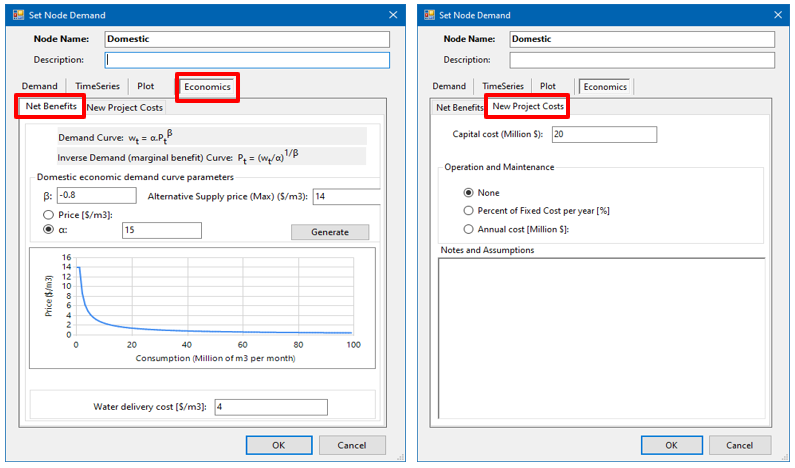
Hydropower Sector

For hydropower projects, the net benefits in each time step is a function of the electricity generated minus the O&M costs. The amount of electric power generated (Pw_t) in period t in watts, is calculated as follows:

Pwt = Ht* qt * η* γ	Eq. 18

Where:

H_t is the average head in meters (vertical distance from water level behind dam to turbines) in period t.

q_t is the water flow (m³/s) through the turbines in period t.

η is the generator efficiency.

γ is specific weight of water (9.807 kN/m³ @ 5˚C) .

The energy generated (E_t) in period t in watt-hours (or kilowatt-hours) is the product of electric power times the number of hours generated. The benefit of the hydropower produced (B_ht) can be estimated by:

Bht = Pt * Et	Eq. 19

Where:

P_t is the average price or marginal value of the electricity produced in period t.

WaterALLOC uses the MODSIM hydropower simulation tool to estimate the power produced by a project based on the average head simulated in the reservoir in each time step, the average flow released, and physical hydraulic capacity through the turbines as a function of the head. The storage and release relationship in the MODSIM solution is driven by system simulated operations for water supply and storage operations, including supplemental water supply and flood control.

Cost-benefit Analysis

The net benefits of water allocation are calculated for each MODSIM node (i.e., demand and reservoir) with economic parameters inputs at run time. For agricultural nodes, the net benefit is calculated for every calendar year, while for the domestic water nodes is calculated every month, and for hydropower is computed every time step. The simulation results include a time series of benefits in monetary terms at these intervals.

With these aggregate net benefit estimates for specified water allocations, the Hydro-economic module can be used to assess incremental or marginal benefits between multiple scenarios. Looking at the change in net benefits between runs, we can analyze tradeoffs and compare the performance of scenarios.

In addition, the results for each node include the option for a time series of project costs on an annual basis. The capital costs are assumed to occur at the beginning of the simulation period and the O&M costs occur each year thereafter for the lifespan of the project, which is assumed to be longer than the simulation period.

To support cost–benefit analysis, the model allows the user to compare the project costs and net benefits with the associated water allocation in three different ways: 1) as present values, discounting the future values in the time series with a user-specified discount rate, 2) as annualized values, and 3) as the total simulated, as the sum of the annual values simulated for each node. A benefit-cost ratio and the net benefit-cost present value are used to compare the assumed benefits and costs, with ratio values greater than one indicating larger benefits than costs.

RTI built a dashboard in WaterALLOC to summarize the benefits and cost results per node and water use type and compare the economic analysis results between multiple scenarios. The figure below shows the dashboard with the main analysis areas and user options. The results displayed in the dashboard include the benefits and cost for the base scenario and each scenario selected, which is displayed in the summary type selected, and a table with the incremental economic benefit between the base scenario and the selected scenarios. The dashboard also includes a graph of each demand node cost–benefit per scenario. The cost–benefit ratio (i.e., BC Ratio) is calculated for each row in the tables, when data are available and adequate for the calculation.

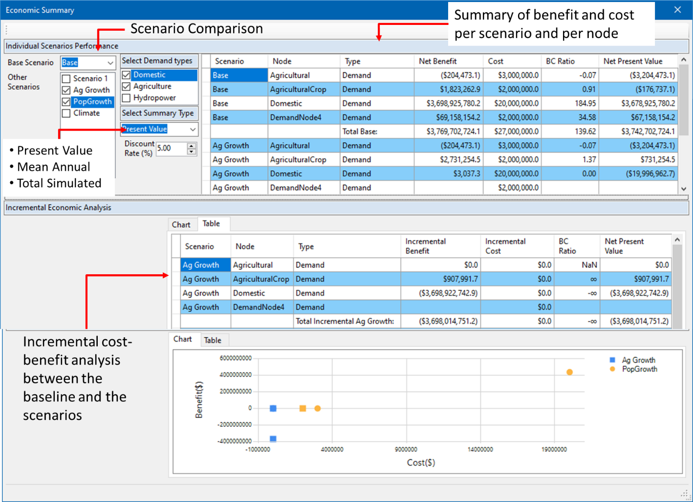
GSFLOW Extension

This extension contains tools to create the MODSIM network for GSFLOW-MODSIM coupled simulation. The main function of these tools is to create a MODSIM network based on the GSFLOW-SFR network. It relies on a shapefile that is created by the Python data processing scripts. The shapefile includes attributes that contain information of the connectivity used by the SFR to move water and is required to link the SFR reaches with the MODSIM links.

The SFR network can contain diversion segments and lakes. Diversion segment could have multiple segments representing different uses or diversion conditions. Flags for storage and non-agricultural use could be set for each of the diversion segments in the shapefile attributes and transferred to the MODSIM links. The SFR shapefile fields include:

Type	Field	Description
Required	ISEG	This field contains the SFR segment number. The segment number is added to the MODSIM link description (“ISEG_###|”) and the number is added to the end of the link name.
	IOUTSEG	Segment number downstream of the current segment
	IUPSEG	This is used to identify diversions. It corresponds to the number of the segments from which the diversion is taken. This number is used to identify the demand node where the diversion segments connect to – when no Demand ID is specified.
Optional	Demand ID	This is an identifier that groups the diversion segments that serve the same place of use.
	Storage Flag	This fields contains an ON/OFF flag that indicates if the diversion has a storage facility to store water diverted in the segment before it is provided to the demand. This field is passed to the description of the MODSIM link representing the diversion segment with the STO: prefix.
	Non-Agricultural	This fields contains an ON/OFF flag that indicates if the diversion serves a non-agricultural type of demand. The value in this field is stored to the description of the MODSIM link representing the diversion segment with the “NONAG:” prefix.

Accessing the Tool

The tool is available in the GSFLOW menu item, when the GSFLOW extension is enabled. The Generate Network item launches the user interface to create the MODSIM network from the SFR shapefile.

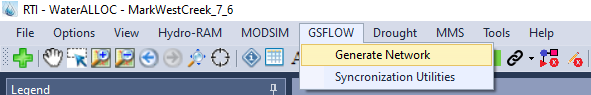
The SFR shapefile should be selected in the configuration setting as the scenario Flowline Layer

The user dialog to map the SFR fields to the information required for generating the MODSIM network provides the names of the key information and the corresponding field in the shapefile (Flowline Layer).

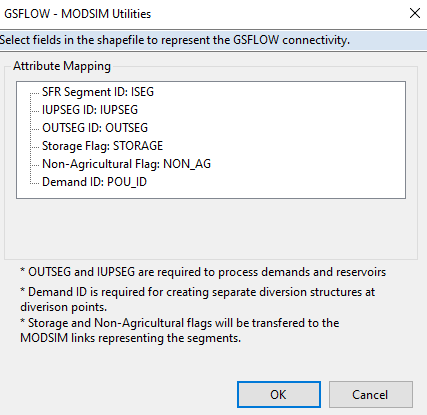
The field names can be edited, selecting the field that would like to be edited, and changing the field name in the dropdown box that shows the available fields.

Expected Outcome

The process creates a new MODSIM network for the active scenario. All the nodes and links in the MODSIM network will be deleted and new links and nodes will be created from the SFR shapefile. The SFR segments in the shapefile are used to create MODSIM links.

Diversions

Since water is diverted from the bottom of the SFR segment, the processing of diversions, creates new nodes at the last part (i.e., last part of the line) of the shapefile line to implement the diversion link, assuring that only water in the segment is available for diversion in MODSIM. The diversion node is named “###_DWS”, using the number of the segment for which the downstream node was created.

Each diversion is created with at least one non-storage node to represent the diversion from the source, i.e., Diversion Inflow Node, that is located at the end of the shapefile line used for the diversion segment.

Demand ID defined: A diversion inflow node and a demand node are created for each Demand ID at the diversion location. The segments associated with that demand are created between the diversion inflow node and the corresponding demand, forming multi-links if multiple segments are associated with the Demand ID. The diversion inflow node is named with “Diversion IDDiversion” and the demand is given the Demand ID name.

Demand ID not defined: a single demand with the name of the IUPSEG is created in this case. All the diversion segments at the current diversion location are implemented between the diversion Inflow node and the demand – a multi-link construct. The name of the demand name is “DEM_IUPSEG#”, and the name of the diversion inflow node is “DEM_IUPSEG#Diversion**“.

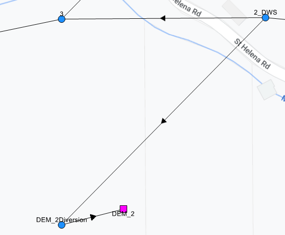
Reservoirs (Lakes)

The python processed shapefile includes connectivity through out the lakes for creating the MODSIM network. In general, negative numbers on the OUTSEG indicates the segment is draining to a lake and the number is associated with the lake number. WaterALLOC creates reservoirs at these locations using the shapefile lines to connect the incoming segments to the MODSIM node and the outgoing segments with the segments downstream of the reservoir.

Operation Optimization Module

• Provide intro to this module and general capabilities. Place holder for now.

Scenarios Management

• Allows set of multiple scenarios for “what if” simulations.

  • Variables that are associated with scenarios

    • MODSIM file

    • HydroBID Settings file

    • Flow Line Layer

• Describe the new scenario options

  • Independent with no data

  • Independent with snapshot of the seed

  • Dependent of the seed

Note: The Flow Line Layer for the new scenario is selected based on the MODISM file base scenario.

Output Visualization

• Explain the different options to explore results (graphs and tables). Provide link to MODSIM documentation.

• Explain the option to compare measured vs. simulated flows and statistical metrics to calibrate the models.

• All MODSIM simulation output is stored in MS Access *.mdb files, which can be directly opened by users if desired. However, MODSIM provides the capability of spatial selection of node and link objects for convenient graphical output display. After a MODSIM run is successfully executed, right-button mouse click on any node or link opens the context menu shown in Fig. 56, but with an added item: Graph, which allows rapid display of output results. Any number of additional nodes or links can be selected, providing comparative display of output results for several MODSIM objects on the same

References

Allen, R.G., Pereira, L.S., Raes, D., and Smith, M., 1998. Crop evapotranspiration-Guidelines for computing crop water requirements-FAO Irrigation and drainage paper 56. FAO, Rome, 300(9), p. D05109.

Allen, R.G., and Pruitt, W.O., 1986. Rational use of the FAO Blaney-Criddle formula. Journal of Irrigation and Drainage Engineering, 112(2), 139–155.

Rineer, J., Bruhn, M. 2013. Technical Note 1. An Analytical Hydrology Dataset for Latin America and the Caribbean. RTI International. Research Triangle Park, NC.

Steduto, P., Hsiao, T.C., Fereres, E. and Raes, D., 2012. Crop Yield Response to Water (Vol. 1028). Rome: FAO.

Help & FAQ

Contact US

Appendix A

Project Database

The WaterALLOC project file (*.waprj) is an database in SQLite format. The database stores information related to:

• Project Info Data

• Scenarios Info

• Scenarios Demand Variables

• HydroBID imported timeseries variables

• MMS Info

The main database tables in the project database are referenced in

[1] [Version 2.4.x] Note that the WaterALLOC interface language should match the language of the heading in the csv output files.

[2] If all households are assumed to have the same household-level demand curve, the aggregate demand is simply the household demand multiplied by the number of households. This also implies that the α parameter for the aggregate demand curve is equal to the α parameter for the household demand curve multiplied by the number of households K.

[3] In the unique case where β equals -1, this equation is undefined, but the benefit calculation simplifies to